

Selected Topics #3:
Graph Neural Networks for Reinforcement Learning
Contents
- Introduction
- Gameplay Football Simulator
- Background: Graph Neural Networks
- Background: Proximal Policy Optimization
- Experiments
- Conclusion
- Sources
- Notation
Learning to Play Football with Graphs and Reinforcement Learning
In this article we’re going to find out how you can train your very own virtual football team by combining the concept of reinforcement learning with that of graph neural networks - and whether you should.
1. Introduction
In late 2020 we participated in the Google Football Kaggle Competition[1], as part of our innovation project at Stuttgart Media University. The objective was to build an autonomous agent that could beat other teams’ agents in a game of virtual football. We chose reinforcement learning to train our agent, and even wrote a blog article about our adventure (German)[2]! During the challenge we brainstormed up a number of concepts for our agent. One rather wild idea was to model the game environment as a graph, to use the given data more effectively. Such an idea isn’t unheard of: There appears to be at least some indication, that graph neural networks can outperform conventional neural networks in reinforcement learning scenarios, on the right data.[3]
In any case, it looked like a good idea - the concept seemed to fit the data really well. But with the challenge deadline approaching, there was little time for proper research, and so we canned the idea and moved on with a more conventional approach, using CNN-like architectures.
After the challenge, though, we started looking through the solutions that some of our former competitors had published (really appreciated!), to validate our own approach and to find out if anyone else had thought of using graphs. Curiously, not a single one of the competing Kaggle teams had even considered it - at least none of the published solutions. That made us curious, because it had seemed so promising when we had first thought about it.
Ah well. Let’s try it ourselves!
Goal
We want to find out if using a graph-based approach has merit in the given reinforcement learning scenario. To this end we will model the game environment data as a graph and train a reinforcement learning agent to perform action-sampling. This will essentially replace the previous CNN feature extractor with a graph neural network. Everything else will remain unchanged, including the reinforcement learning specific artefacts.
Agenda
Let’s start with a general look at the GFootball environment. After this we will briefly cover the necessary theory behind graph neural networks (GNN), graph convolutional networks (GCN) and the proximal policy optimization algorithm for reinforcement learning (PPO). The goal is to give you, the reader, an idea why we chose those particular technologies and methods.
We will then design our own training setup and conduct experiments based on that, before finally evaluating how well our initial ideas hold up.
2. Gameplay Football Simulator
GFootball Environment
With their GFootball[5, 15] environment , Google has created a highly flexible and realistic football (soccer) simulator, that is based on the common rules of football (red and yellow cards, offside etc.). It offers a selection of different game modes (kick-off, free kick, throw-in, penalty kick etc.) and even models each player’s level of exhaustion.
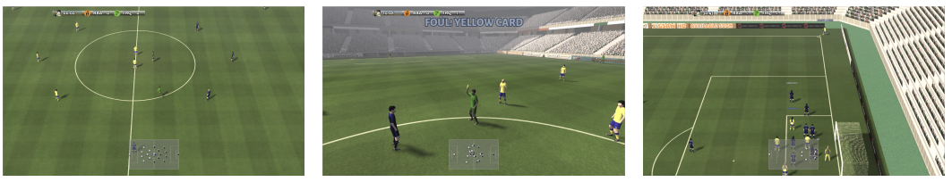
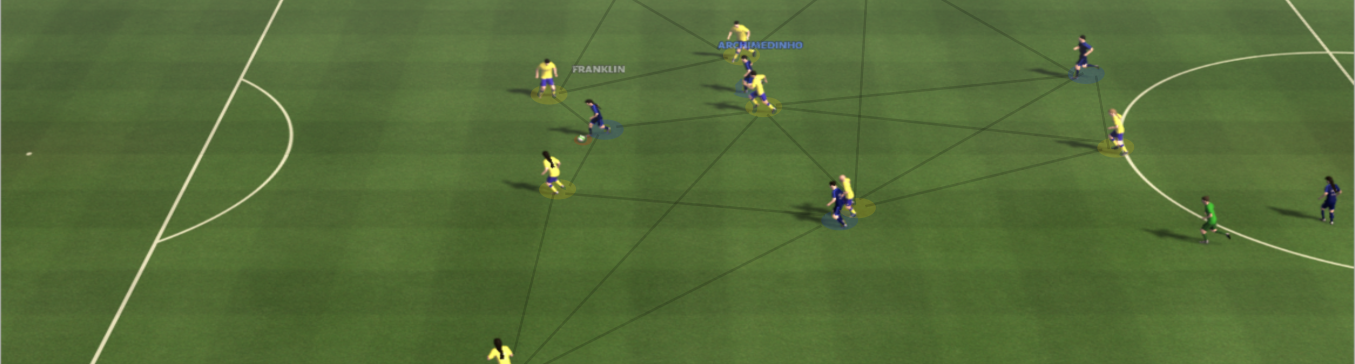
Over 19 different actions can be used to control one or multiple players (8 movements, 3 passes, goal shot, sprint, tackle etc.). The simulator offers a very simple interface that is compatible with OpenAi’s Gym Toolkit [4] specification. Through interaction the simulator returns a plethora of information about the current playing field. This information is represented in a number of different formats. The current game situation (state) can be returned as numeric values (players’ and ball’s coordinates, movement directions, tiredness factor, ball ownership etc.) or through images (players and ball are single pixels). The following GIF shows a game setting as it may happen in the simulation. Here our agent can only control one player (active player), the one that owns the ball (attack) or is closest to it (defense).
Based on the chosen actions, the simulator’s feedback contains both a representation of the game’s new state and a reward value. The most straightforward reward mechanic is a reward +1 for a scored goal and -1 for a goal scored by the opposing team.
Speaking of which, the simulator also includes a built-in bot opponent with continuously adjustable difficulty. Players can challenge the built-in bot either manually through keyboard input or via an agent that they developed.
The high level of configurability also allows for special scenarios (e.g. attack or defense only), other opponents (rule-based AIs or even trained agents) and custom reward functions (e.g. +0.1 for ball ownership).
The official documentation can be found on GitHub[5].
Built-in Opponent
By default the opposing players are controlled by a bot introduced in the GameplayFootball simulator[6]. The difficulty can be set continuously between $0$ and $1$ . Predefined levels are easy ($0.05$ ), medium ($0.6$ ) and difficult ($0.95$ ). By default, only one player is controlled at a time - the one with the ball on offense, or the one closest to the ball on defense. The non-active players are controlled by another simple rule-based bot that follows reasonable football actions. The flexibility of the simulator allows multiple models to be configured per team and complex multi-agent scenarios to be built. However, in this article we will focus on the case of controlling only one player. We also only train against the bot on the easy setting, but we could always increase the difficulty in the future.
State and Observations
An environmental feedback consists of four elements:
observation, reward, done, info = step(action)
- done is true whenever an episode ends
- info holds some debug information and the final score
- reward signal
- observation depends on the representation.
There are three default representations available for the observation:
- Pixels: Pixel representation of the game screen, downscaled to $72 \times 96$
- Super Mini Map (SMM): Simplified spacial (mini-map) representation of a game state. It consists of several $72 \times 96$ planes of bytes, filled in with zeros except for positions of the players and ball:
- Floats: Simplified representation of a game state encoded with $115$ floats
- Raw: Dictionary with all the information the environment offers.
Raw Observations:
- Ball information:
ball coordinatesball_directionball_rotationball_owned_teamball_owned_player
- Left team (for each player):
left_team coordinatesleft_team_directionleft_team_tired_factorleft_team_yellow_cardleft_team_activeleft_team_roles
- Right team (for each player): same as the left team
- Controlled player information:
active- {0..N-1} integer denoting index of the controlled players.sticky_actions- e.g. sprinting is active as long as the action release_sprint is triggered
- Match state:
score- pair of integers denoting number of goals for left and right teams, respectively.steps_left- how many steps are left till the end of the match.game_mode- current game mode, one of:NormalKickOffGoalKickFreeKickCornerThrowInPenalty
Actions
19 actions are available, of which
- 8 are movement actions (left, top left, top, top right, right, bottom right, bottom, bottom left)
- 4 are pass/shoot actions (long pass, high pass, short pass, shot)
- 1 is the idle action
- 6 are other actions (sprint, release direction, release sprint, sliding, dribble)
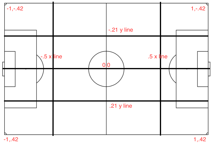
Visualization of the field
Have a look at the game field coordinates:
Rewards
By default the environment returns +1 for shooting a goal and -1 for an opponent’s goal. Because the scoring reward can be hard to observe in the initial stages of a training process, the developers add a checkpoint reward - that’s a reward of +0.1 given when the player (with the ball) enters one of $10$ checkpoint regions of the opponent’s field for the first time. This reward is only given once per episode to avoid reward exploitation.
Choosing a Graph Representation for the GFootball Problem
Recall the common structure of many deep NN architectures:
- A feature extractor takes whatever input data we give to the network and turns it into an abstract representation, usually a one-dimensional vector. The exact architecture of the feature extractor is largely dependent on the way in which that data is represented (images, time series, text, graphs etc.). The feature extractor can be shallow or become up to several hundreds, even thousands of layers deep.
- A classifier (usually the last hidden layers of a deep neural network) takes the resulting representation and performs some desired operation, e.g. a class mapping or regression. In our case, we will feed the abstract representation into our reinforcement learning agent to predict different values (more on that later). It only makes sense that the type of the given data affects the choice of architecture, especially for the feature extractor. The choice comes down to a mix of obvious markers (e.g. the broad domain) and the developer’s domain knowledge. Are you working with image data? You will likely want to choose a convolutional neural network. Time series data? Recurrent architectures and LSTM come to mind. Building a language model? Perhaps attention is what you need.
Comparing the four different data representations in the GFootball environment, there are essentially two types of data available: Numeric values and images (spatial values). The simplified representation is just a $115$ -dimensional vector. One or two fully connected layers can make short work of that. For the two image based representations (full images and SMM), a CNN feature extractor is the obvious first choice. Both methods, CNN and MLP, come with reference-implementations that worked just fine for us.
But what about the raw representation? As it turns out, the raw observation data might lend itself really well to a graph representation: You have $11$ players on each team plus a ball. That makes $23$ entities (nodes) that each have their own set of properties (plus a few globals). As they interact during a game, they also have relations to each other. We can think of a few possible advantages that this representation has over the other two methods:
Advantage: Sparsity
One issue with CNN and GFootball is that image-encoded information is extremely sparse. Take the SMM format: The interesting pixels are white (players, ball), all other pixels are black. The vertices that actually hold meaningful information are few and far between, while the vast majority of pixels in the SMM images holds no information at all. The CNN doesn’t know this and dutifully traverses the entire image, wasting precious GPU cycles in the process.
Instead of using a sparse image, we will be building the input graph ourselves, using the raw observation data provided by the environment. This graph, in contrast to the SMM images, will not be sparse.
Advantage: Shared Weights
A graph convolutional network can take advantage of the concept of shared weights, just like a regular CNN does. Instead of a large MLP that takes hundreds of input features, the parameterized functions in a GCN take features node by node, player by player and could require much smaller input-vectors.
Advantage: More Information
Surely we could just take the raw representation, flatten it and pass it through an MLP just like the simple representation. However, we would lose the associations of which feature belongs to what player - just to maybe relearn it later. A graph-based approach could retain this information.
In addition, we can draw on our own domain knowledge and encode information directly into the graph topology. This includes high-level information that is present in the raw data representation (A ball is not a player and has different features associated with it.) or even new information that is not in the raw data (The agent should place more importance on the players closer to the active player.).
3. Background: Graph Neural Networks
This is our first foray into the world of graph neural networks (GNN), so we will cover some of the basics first. There are many excellent tutorials out there that explain the ins and outs of the graph neural networks[7] and specifically graph convolutional networks[8], which we use here. For the sake of brevity, we will not reiterate their contents, but rather establish a common notation:
$G$ is a directional graph with nodes and edges: $G=(V,E)$ , where $V$ is the set of all vertices (nodes) $n$ and $E$ is the set of all edges $(n_i,n_j)\in{E}$ . An edge that starts and ends in the same node is called a self-connection.

NB: Graph neural networks are not a rigidly defined concept. GNN is really an idea that can be implemented in many ways and with multiple degrees of freedom. By making any assumptions about our graph, even by using methods such as message passing, we are already making design decisions. The methods we chose and that are explained below are likely not the only possible, valid approach. We made these choices based on two factors: By the popularity of the methods and by our intuition of what a meaningful graph representation of the given data would look like.
Message Passing and Graph Convolutional Networks
A graph convolutional network is a special concept for a graph neural network. Among others, it uses a mechanism called message passing. This mechanism allows each node in a given graph to receive information about its direct neighbors[9].
The hidden state $H$ of a GCN contains the states of all nodes $n\in V$ . Information can be passed between any two nodes $(n_i,n_j)$ through edges. $A$ holds the information which node is connected through an edge to which other node. It is often modeled as an adjacency matrix. The dummy graph in the example above is fully meshed and has self-connections, its adjacency matrix would look like this:
$$ A = \left( \begin{matrix} 1 & 1 & 1 & 1 \\ 1 & 1 & 1 & 1 \\ 1 & 1 & 1 & 1 \\ 1 & 1 & 1 & 1 \end{matrix} \right) $$In a GCN layer, both node states $H$ and adjacency information $A$ are fed to some parameterized, nonlinear function. The function then returns a new hidden state ($t$ is the layer index):
$$H_{t} = func(H_{t-1},A)$$NB: Another option to model adjacency information is to define $A$ as a list of edges $n_j \rightarrow n_i$ . Both representations contain the same information, but the list option is more memory efficient when dealing with large, sparse graphs. In such a case an adjacency matrix would become quite large but contain mostly zeros.
Message Passing in Detail
Let’s take a look inside the message passing operation. We will consider two parameterized functions inside a GCN layer: $f$
and $g$
. Every node $n\in{V}$
has its own hidden representation $h^n_t$
, a vector. Each $h^n_t$
corresponds to a row in $H_t$
.
Function $f$
takes the states of two adjacent nodes and returns an edge representation $e_{ij} = f(h^{n_i}_{t-1}, h^{n_j}_{t-1})$
with $n_i\neq n_j$
. Edges are considered directional, meaning that information flows from $n_j$
to $n_i$
. We call $n_j$
the source and $n_i$
the target node.

For every edge that connects some neighbor node $n_j$
to the current target $n_i$
, both $h^{n_j}$
and $h^{n_i}$
are passed through $f$
. All resulting edge representations $e \in \tilde{E}$
are then combined using some function $u_f$
. This can be any type of commutative combination, the choice is up to the developer:1
Finally, the resulting aggregate is passed through $g$
. The resulting node state $h^n_t$
is now ready to be passed to the next layer. Considering the current node $n_i$
, the message passing operation can be expressed through the following notation:2
Note that we don’t just feed the aggregate to $g$ , but also the node’s previous state, gained through the self-connection. If we didn’t do that, any new node state would completely overwrite the node state from the previous GCN layer. This would not be ideal, because that information may be important. Since $g$ is parameterized, it is now up to the neural network which information is more important: Its previous state or its relations with its neighbors.
NB: We found GCN setups, in which $f$ only takes the source node representation, but not the target one. However, we had no success with this approach.
The figure below shows how the message passing operations ($f$ , $g$ and $u_f$ ) are positioned w.r.t the input graph.

NB: NN layer $f$ may also take some edge-specific information as well, but we’ve left this out to avoid confusion, because we don’t do this. In addition, we have omitted the activation functions $\phi_f$ and $\phi_g$ from the notation to improve readability. We have also left out the layer parameters (weights) $w_f$ and $w_g$ for this reason. Just in case, a full notation table can be found at the end of this notebook.
1 We encountered some very interesting behaviors with some types of aggregation. See the experiment section for more details.
2 The notation has been inspired by an online lecture by Microsoft Research[10]. However, we define any commutative combination functions as $u_f$
and $u_g$
, instead of using a union operator.
Why Graph Convolutional Networks?
The concept behind a GCN is similar to the local receptive field in convolutional neural networks: Each node of a GCN layer only receives edge information about its immediately adjacent neighbors. Information from beyond this receptive field may only reach it in the GCN layer after. The larger the graph grows, the deeper it must be to receive information from nodes that are farther (more edges) away.
If this process reminds you of the image convolution in the popular CNNs, that’s no accident. In fact, CNNs can be interpreted as highly specialized graph neural networks. One only needs to imagine a pixel image as a fully meshed graph where every pixel corresponds to a vertex. Consider the following figure:
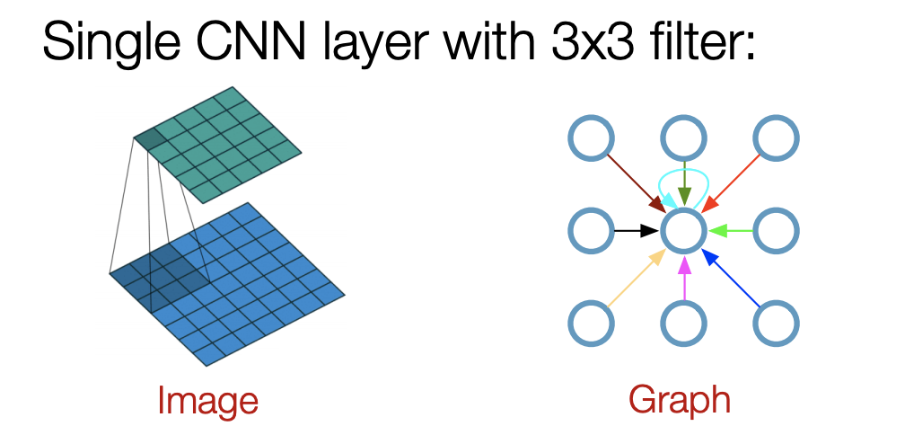
That said, our specific graph is really, really small. One GCN layer is likely enough to inform every node about all other neighbors. This means we might not leverage all of the features a GCN offers.
Still, GCN have some more handy properties that help us: Since we have to construct the input graph ourselves from raw data, it is helpful to have a GNN architecture that is indifferent towards the graph topology. This way we will be able to try different topologies later on without having to rewrite the entire GNN.
Additionally, the concept of shared weights still applies, so that we don’t need a different set of weights for every single node either.
4. Background: Proximal Policy Optimization
The goal of this article is not to explain the underlying reinforcement learning algorithm in detail. We will briefly introduce the proximal policy optimization[16] (PPO) method and focus on the essentials. Furthermore, we assume an understanding of the terms policy, reward, state-action - and (state-) value function. If any of these terms sound unfamiliar to you or if you prefer a more in-depth explanation of the algorithm, you may want to take a look at these great lectures[11]. We also recommend the book on reinforcement learning by Sutton & Barto[12]. Both are used as reference for the following section. Fortunately, we didn’t have to implement the PPO algorithm from scratch ourselves. The company OpenAI provides a framework for reinforcement learning - the OpenAI Baselines[13].
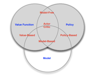
The PPO can be described as a
- model-free
- on-policy
- actor-critic based
reinforcement learning algorithm. Let’s take a closer look at these features:
RL Taxonomy
Algorithms can be either model-free or model-based: In model-based algorithms, the agent has access to (or learns) an accurate model of the environment’s dynamics (state transitions and rewards). Having a model allows the agent to plan, because it knows the characteristics of the environment and therefore can think ahead and sees what would happen for a range of possible choices. A famous example is AlphaZero. The model-free approach does not attempt to explicitly understand the environment by first learning a model of the underlying dynamics. Instead, the algorithm simply gains experience by interacting with the environment to (hopefully) determine the optimal strategy. Besides the PPO algorithm, the well-known Q-learning algorithm and its variants also belong to the model-free approaches.
Algorithms can be either off-policy or on-policy: Let’s say we want to optimize the target policy $\pi_{target}$ . For this, the agent collects data by interacting with the environment and chooses actions according to behavior policy $\pi_{behave}$ . In off-policy learning, $\pi_{behave}$ differs from $\pi_{target}$ . Take Q-learning: We want to optimize a greedy policy (given a state, we always choose the action that maximizes the value-function), but in order to gain experience, the agent follows a $\epsilon$ -greedy policy - ☝️ that makes two different policies! In on-policy algorithms like PPO, $\pi_{behave}=\pi_{target}$ . Here, $\pi_{target}$ can be roughly seen as a list of action probabilities, i.e. we follow $\pi_{target}$ to collect experience, which is then used to make actions more or less likely by modifying the values in $\pi_{target}$ .
Algorithms can be value-based, policy-based or actor-critic based: The former does not directly learn a policy but rather a value-function from which the policy can be derived. Like in Q-learning, we try to learn a function that predicts how good an action might be, given a state, by calculating the expected reward. The policy can then be derived by always choosing the action that maximizes this function. In contrast, policy-based algorithm learn the policy itself. There is no value or state-action function. To combine the advantages of both, actor-critic methods have been introduced: The policy is learned directly without having to derive it from a value function (policy-based). However, to evaluate the policy and the actions chosen with it, a value function is learned (value-based).
Objective
PPO attempts to maximize the long-term reward by minimizing a loss function $L_{total}$ (inverse of the objective function):
where $\theta$ annotates the parameters of our underlying models.
$L^{CLIP}(\theta)$ is called the clipped surrogate objective and is calculated by dividing the probability of an action $a$ under the current policy by the probability of $a$ under the old (previous) policy. This ratio is then multiplied with the so-called advantage. The advantage function captures how much better an action is compared to the average of all rewards (caused by all possible actions taken) at a state $s$ . Without any constraint, maximizing this result would lead to a huge policy update. In order to ensure that $\pi$ doesn’t change too much, the ratio is clipped.
$L^{VF} (\theta)$ is the value-loss. It’s the squared difference between the current state value and the target value. The target value is high if the sampled action gives us a high advantage.
$S$ denotes an entropy bonus. Entropy ensures exploration because the more evenly distributed the actions in our policy, the higher the entropy and the smaller $L_{total}$ .
Thats it! We compute the gradient w.r.t. the model parameters $\theta$ and (hopefully) increase the reward! Let’s have a closer look at the mechanisms.
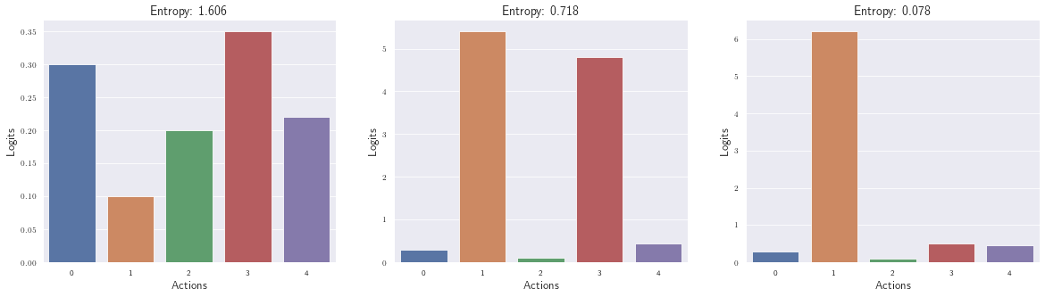
Exploration
There is a risk of premature convergence that leads to one action probability dominating the policy, thereby preventing exploration. This is prevented by the introduced entropy coefficient. It’s like a regularizer: Maximum entropy is reached when all actions are equally likely, minimum entropy is reached when one action with the highest probability dominates the policy. The entropy is calculated based on the actor’s logits (can be seen as $\pi$ ). Since entropy is a negative factor in the loss function, a higher entropy is good for keeping the loss small. The following figure puts different distributions and entropy in context. See how entropy shrinks when one action begins to dominate.
Action Sampling
In deep learning we often want to sample discrete data. The same applies to the present RL task, as we need to sample actions from a categorical distribution (19 actions). The usual way would probably be to pass the logits through a softmax function and sample from the created distribution with np.random.choice or tf.multinomial. However, a more efficient method for drawing samples from categorical distributions has become established by sampling from a discrete distribution parametrized by the unnormalized log-probabilities - this is the so called Gumbel-max trick. OpenAi makes use of that in their baseline implementation. Let’s see how this is reflected in the code:
def sample(logits):
    x = tf.random_uniform(tf.shape(logits))
    return tf.argmax(logits - tf.log(-tf.log(x)), 1) # noise = -tf.log(-tf.log(x))
It makes sense, doesn’t it? Without the added noise, the argmax operation would always return the index of the biggest logit. This is not really what we want, because that would be more like the way we select actions in value-based algorithms. Therefore, we add noise to the logits, to add some stochastic element. But why not just using noise? Why taking the negative log twice -tf.log(-tf.log(x))? The exact explanation would exceed the scope of this article, but suffice it to say that the described sampling process only works if the noise is sampled from a specific distribution - neither uniform nor normal, but from the so-called Gumbel distribution. If you are into proofs and maths, check out the work on The Gumbel-Max Trick for Discrete Distributions[17].
Let $\pi$ be our current policy. We can draw a sample by computing $a= argmax_i(log(\pi_i)+noise_i)$ , where $noise_i \sim Gumbel(0,1)$ . We’re almost there! We can compute $noise_i$ by using samples $x_i$ from a uniform distribution: $noise_i = -log(-log(x_i))$ and boom, we have derived the action sampling method as used by OpenAI.
To illustrate that Gumbel-noise really works best, here is an example:
# first create a dummy categorical distribution with 5 action
cats = 5
probs = np.random.randint(low=1, high=20, size=cats)
probs = probs / sum(probs)

# apply log
logits = np.log(probs)

# add uniform-distributed noise to logits
def sample_uniform(logits):
    noise = np.random.uniform(size=len(logits))
    sample = np.argmax(logits + noise)
    return sample

# add normal-distributed noise to logits
def sample_normal(logits):
    noise = np.random.normal(size=len(logits))
    sample = np.argmax(logits + noise)
    return sample

# add gumbel-distributed noise to logits
def sample_dg(logits):
    noise = np.random.uniform(size=len(logits))
    return np.argmax(logits - np.log(-np.log(noise)))

# compute action probabilities from 5000 sampled actions
def get_estd_probs(s):
    estd_probs, _, _ = hist(s,
                        bins=np.arange(cats + 1),
                        align='left',
                        edgecolor='white',
                        density=True)
    return estd_probs

# Sample 5000 actions based on the logits
n_samples = 5000
samples_u = [sample_uniform(logits) for _ in range(n_samples)]
samples_n = [sample_normal(logits) for _ in range(n_samples)]
samples_gd = [sample_dg(logits) for _ in range(n_samples)]

# estimate distribution based on samples
estd_probs_u = get_estd_probs(samples_u)
estd_probs_n = get_estd_probs(samples_n)
estd_probs_gd = get_estd_probs(samples_gd)
Plot the estimated probabilities and compare them to our original ones. (We’ve also added the KL-divergence to measure the distance between the distributions.)
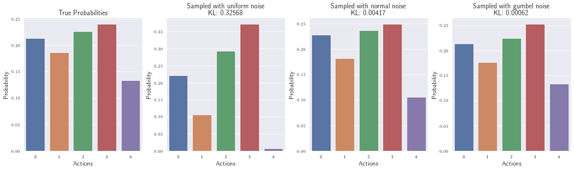
Normal distributed noise works better than uniformly distributed noise, but with the Gumbel noise we get a similar distribution compared the the “original” one (also seen from the small KL divergence).
NB: There is actually another advantage of using the Gumbel distribution: ☝️
Approximating the argmax function (which is not differentiable) by a softmax function leads to a chain of derivable operations that allow you to compute the gradient over the action sampling process (might be required for backpropagation). However, as the code snippet above shows, this is not used in the baseline implementation. Instead, they use another neat trick in order to stay differentiable. The sampled action is used to create a one-hot vector, which in turn is used as a label to calculate the cross-entropy (after applying softmax). Because the label is only ≠ zero at one index, the cross-entropy boils down to the negative log probability of the action. This leads to the fact that the process of action sampling is not included in the formation of the gradients and therefore does not have to be differentiable.
You may now rightfully ask: Why do we present the action sampling in so much detail?
During our experiments we encountered an unstable training behavior that we believe is at least partially influenced by the way actions are sampled. Since we really went off on a tangent there, we felt that we wanted to include our findings. More on this in experiment 4.4.
5. Experiments
During our investigation of the applicability of GCN as feature extractor for RL tasks, we have conducted many different experiments. To keep this article “short”, we will focus on the most important ones. For each experiment, we first develop a simple hypothesis that motivated the experiment. This is followed by the evaluation, i.e. what we observed and how we interpret that.
For the present reinforcement learning task and under otherwise identical training conditions,
comparing a GCN feature extractor on graph input data with GFootball's default MLP feature extractor on flat input data:
$\mathcal{H}$ = The graph representation can achieve a greater total reward, or the same reward but with fewer model updates, compared to a multilayer perceptron with similar complexity.
NB: Don’t confuse the hypothesis symbol $\mathcal{H}$ with the latent state of a GCN layer $H$ ! ☝️
5.1 Training Setup
We’ve already established that we are using a GCN architecture in combination with the PPO algorithm for reinforcement learning. The input data dimension is $23$ nodes times $43$ features per node. The resulting NN architecture (does not refer to the topology of the graph) used in all experiments is as follows:

You may notice two differences from the earlier example architecture: Most importantly, the output of the single GCN layer is fed into the computation of the policy and state value. Second, there is now a new aggregation function $u_g$ , that governs how the GCN state $H_1$ is treated.
Let’s look a bit closer at $u_g$ . Recall how message passing occurs between the nodes: Each node is updated with the information of its incoming edges and receives a new representation $h^n_1$ . Once this information leaves the GCN layer, the node information is passed through $u_g$ . This function may be designed in a number of ways: Either the entire $H_1$ is aggregated (mean) or flattened into a long vector. Perhaps all information $H_1$ is even discarded, except for the node state of the active player, $h^{n_{act}}_1$ - this is a design choice, just as with $u_f$ .
The complete creation of the PPO input representation can be described with the following notation:
Or in pseudocode:
for n in nodes:

    for n_j in nodes adjacent to n:

        # get edge representation f(n, n_j)

    # combine edge representations using u_f,
    # get new node representation g(self-connection, u_f(...))

# combine node representations using u_g

# pass info to the policy and value functions
NB: As you may notice, there is only one GCN layer present. This choice was made early on. The assumption here is that we don’t need a deeper message passing structure, because our graph is going to be very small and can easily be explored fully within a single layer. Deeper GCN are rather useful when there are huge graphs. What this architecture cannot cover is the concept of increasing levels of abstraction also found in CNNs, but that would likely require a larger graph.
The policy and value functions are provided by the OpenAI baselines and were not modified. Since this project is not an exercise in hyperparameter optimization, we followed OpenAI’s optimized hyperparameters closely. These can be found here. To speed up training, we used $20$ environments running in parallel instead of the proposed $16$ . Other deviations are explained per experiment, if applicable. Trainings were stopped after $150M$ steps at the latest. This was a practical choice to keep training times manageable. With a step size of $512$ and $20$ environments, this results in about $15.000$ update loops and takes 3-4 days of training based on our hardware.
5.2 Build a Baseline
Any meaningful investigation needs a baseline, to put the achieved results in relation. The motivation of this work was to investigate whether the use of graph structures leads to better feature vectors compared to a more conventional approach, using a multi-layer perceptron. Therefore we build our baseline with a two-layer MLP, as it’s already implemented in the baseline repository. As a measure of quality, we considered the total reward and how fast it was achieved. Instead of looking at the reward after each episodes, we considered the average over the last $100$ values. We’ve mostly concentrated on using either $64$ neurons or $512$ in order to investigate the influence of the model complexity. This leads to two MLP baseline architectures:
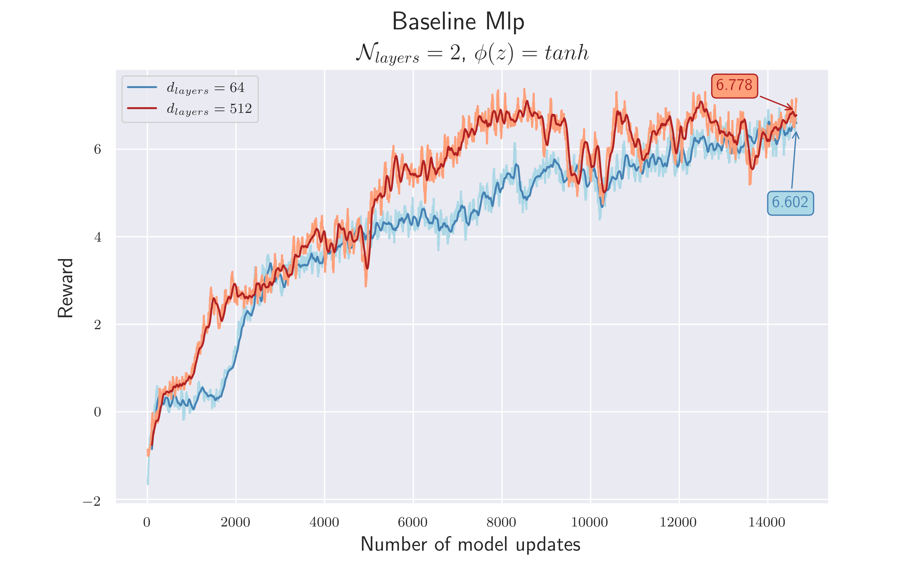
After $150M$ game-steps, both architectures achieve a similar total reward of about $6.7$ . The higher complexity does not seem to affect the amount of reward, but it does affect the speed at which it is achieved.
5.3 Getting Started with Graph Neural Networks
When modeling the raw numeric data as an input graph, we need to assign it some topology $\mathcal T$ . As a first, naive approach, the input graph is simply modeled with fully meshed topology. This lets us stay as close as possible to the baseline. Other options for $\mathcal T$ will be explored later.

Since there are many degrees of freedom in how to implement a GCN, the first priority was to find a suitable combination of hyperparameters. In addition to the fully meshed topology, we also used the same kernel-initializers as the MLP and used $64$ output neurons for $f$ .
While at it, we performed a first experiment to evaluate the validity of our architecture: For $u_g$ we had the option to concatenate the node representations (flatten), or to simply take their average. Our bet was on the former, since we thought that too much information is lost this way - especially the ball information. The flatten operation gives more flexibility and allows the network layers after it to combine the node states by itself.
This is the first real GCN experiment, outlining the general feasibility of our idea. We assume that:
$\mathcal {H_1}$ = Using a graph neuronal network as feature extractor is usable in combination with RL tasks.
$\mathcal {H_2}$ = Using a concatenated vector of all updated node representations leads to better performance than taking their average.
Function $f$ and $g$ output a $64$ -dimensional feature vector that runs through a $tanh$ before the aggregations take place. Feature vectors, belonging to edges that flow into a node, are summed up. A distinction is made between $u_g=mean$ and $u_g=flatten$
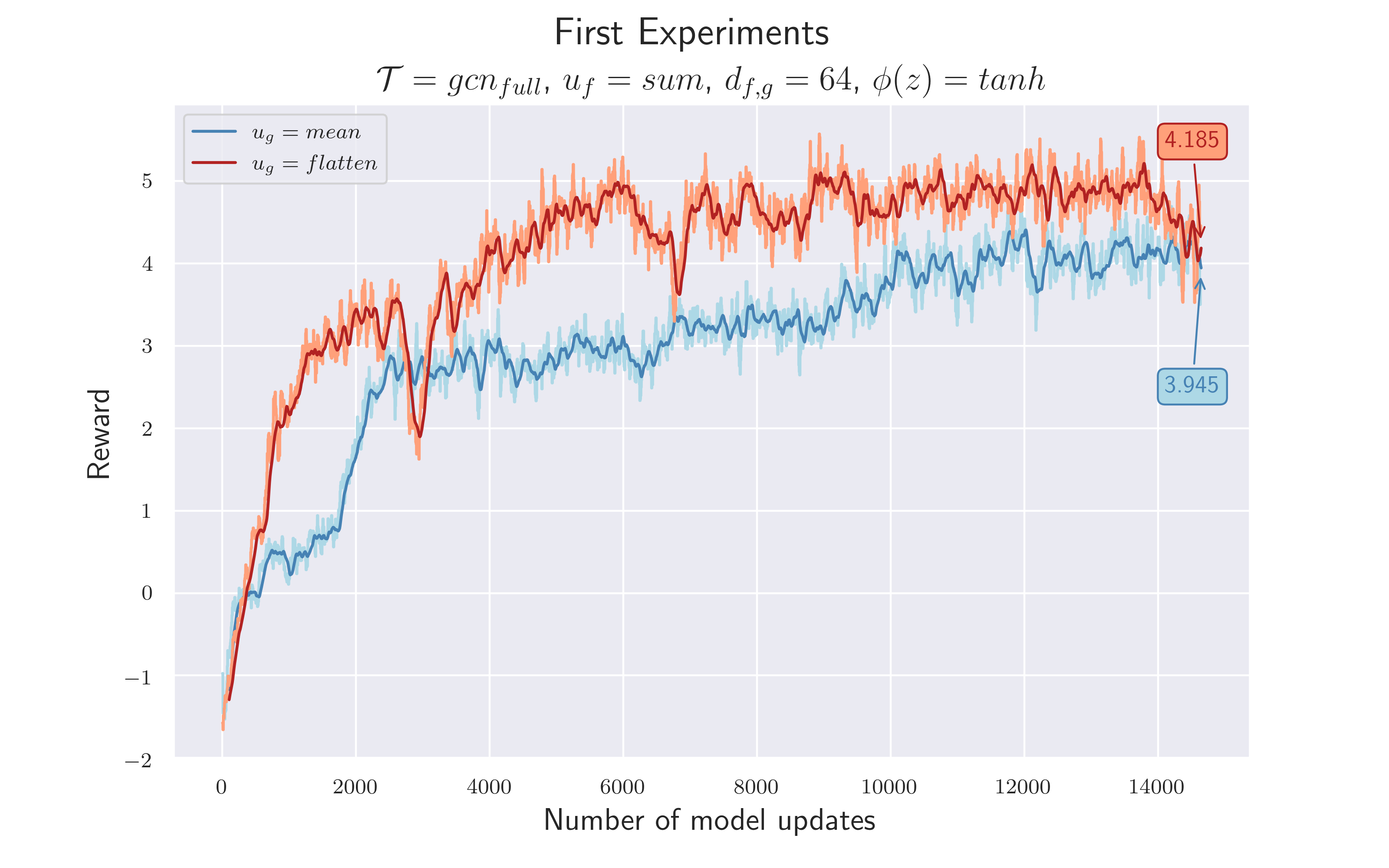
Since we clearly saw a learning effect, we considered $\mathcal {H_1}$ to be confirmed. Two more conclusions could be drawn:
- The experiment confirmed $\mathcal {H_2}$ . Using $u_g=flatten$ led to a better performance. Besides the higher total reward, it could also be deduced that concatening the node states led to a faster training process, since the red line is almost always above the blue line. However, there is only a marginal difference between the rewards at the end of the training, which suggests that both approaches work in principle.
- Compared to the baseline, the performance of this first GCN architecture is lower. Although intermediate results showed a reward $> 5$ , the final difference between the rewards compared to the baseline is about $2.5$ . This has indicated that either we have not yet found the right hyperparameters or it would require more complexity to extract information from the graph structure.
5.4 Increasing Model Complexity
To investigate the influence of the model’s complexity, the number of the output neurons $d_{f,g}$ was increased to $512$ .
An output dimension of $64$ might be too small to capture the complexity of the graph structure, which in current topology includes $23*22=506$ edges and $43$ features as $h_0$ . Increasing the output dimension of $f$ and $g$ allows the network to encode more useful information about the players and the ball. Therefore, the performance should increase.
$\mathcal {H_3}$ = More complexity is needed to extract useful information from the connection between nodes. In addition, other hyperparameters might be more suitable than the current ones
The hyperparameters from the previous best run are left the same, except for $d_{f,g}$ , which is set to $512$ . Since the first hypothesis has been confirmed, albeit not very strongly, we choose $u_g=flatten$ .
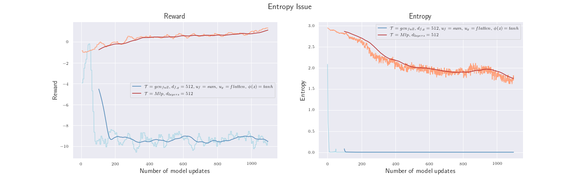
We stopped the training after $1000$ model updates because we were faced with some strange training behavior. The left plot compares the reward of our model an the corresponding baseline. The reward drops to $-10$ and does not recover. That made us wonder, especially when we realized that the entropy (right plot) drops almost to zero. It seems like one action dominates the policy.
5.4.1 Tangent: Investigate Falling Entropy Problem
NB: This section gets quite technical. If you’d prefer to skip this part, you may jump straight to experiment 5.5.
Decreasing entropy is a good thing, it is what you would expect because the algorithm gains experience during training and therefore prefers certain actions - but such a rapid and sharp drop in the entropy value is certainly not correct. The naive approach of increasing the entropy coefficient (by a factor of ten) and thus forcing the algorithm to explore on a larger scale was not successful. Therefore, we conducted further experiments and found four hyperparameters that seemed to affect the falling entropy problem:
- the dimension of the final feature vector that is passed to the actor and critic. Can be controlled with $d_g$ and $u_g$
- the aggregation $u_f$ over the edge-related feature vectors (sum or mean),
- the learning rate and
- the activation function
We then decided to get to the bottom of the problem and investigate the falling entropy problem in more detail. To do so, we integrated tensorboard and monitored
- the sampled actions ($Hist_A$ ),
- the final feature vector (called latent vector) that is passed to actor/critic ($Hist_{FV}$ )
- the policy (logits) itself ($Hist_{\pi}$ ) and
- different weights ($Hist_w$ ).
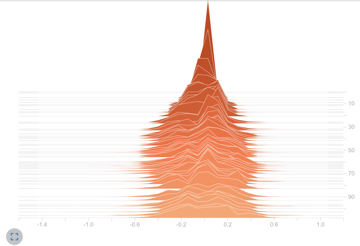
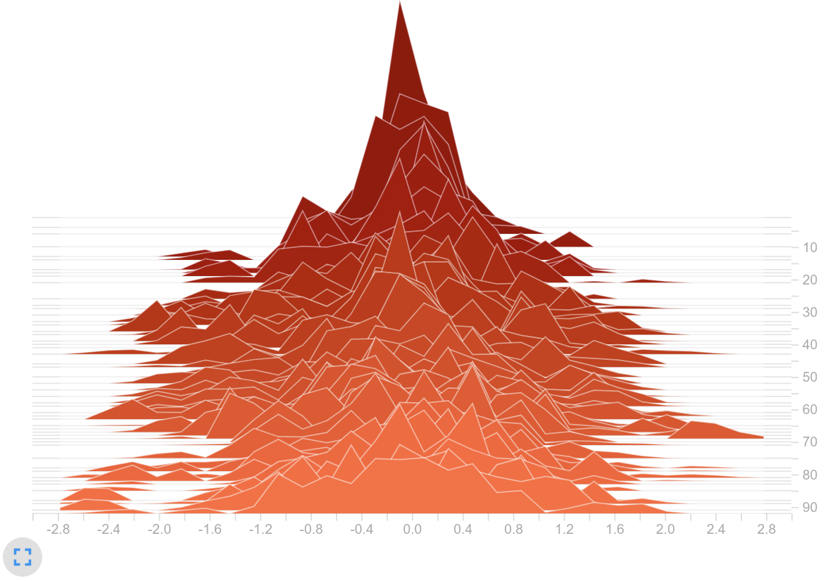
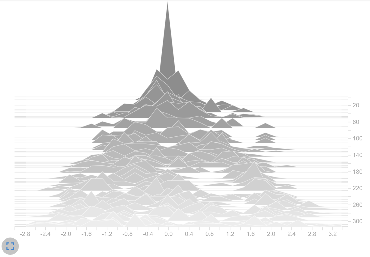
The following histograms compare the distribution of the selected variables between the 512-MLP baseline (orange) and the current GCN (from 4.4) in green. We start with $Hist_{FV}$ .
Histogram of latent vectors
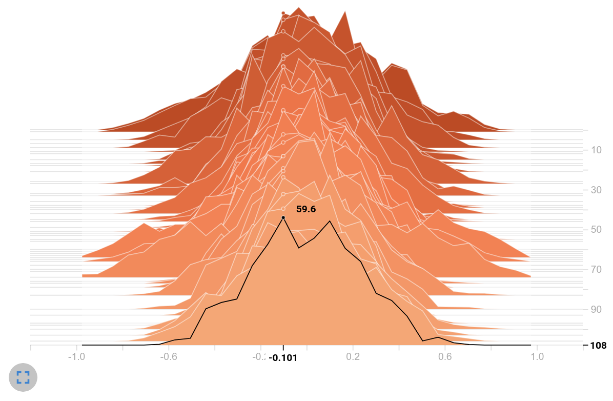
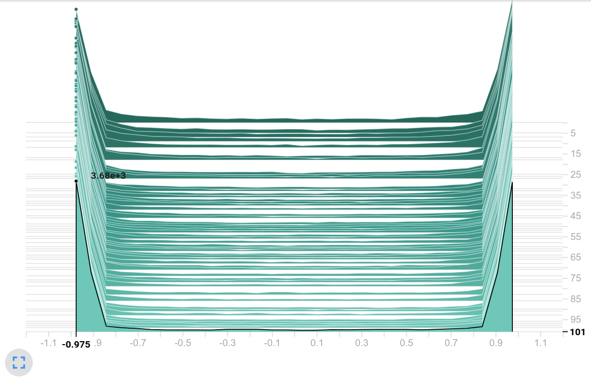
Observation: Both models use the tanh as an activation function. Therefore the histogram ranges from $-1$ to $1$ . However, the histogram on the right shows the majority of the values close to these interval limits - most of the values lay inside the saturation area of tanh. Moreover, the frequencies on the right are by far larger compared to the histogram values of the baseline.
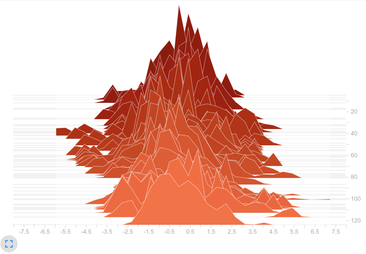
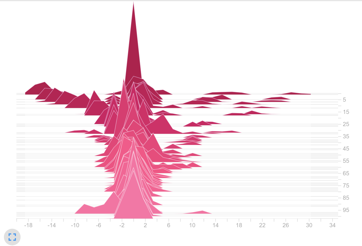
We move on to the policies (logits):
Policy values (logits)
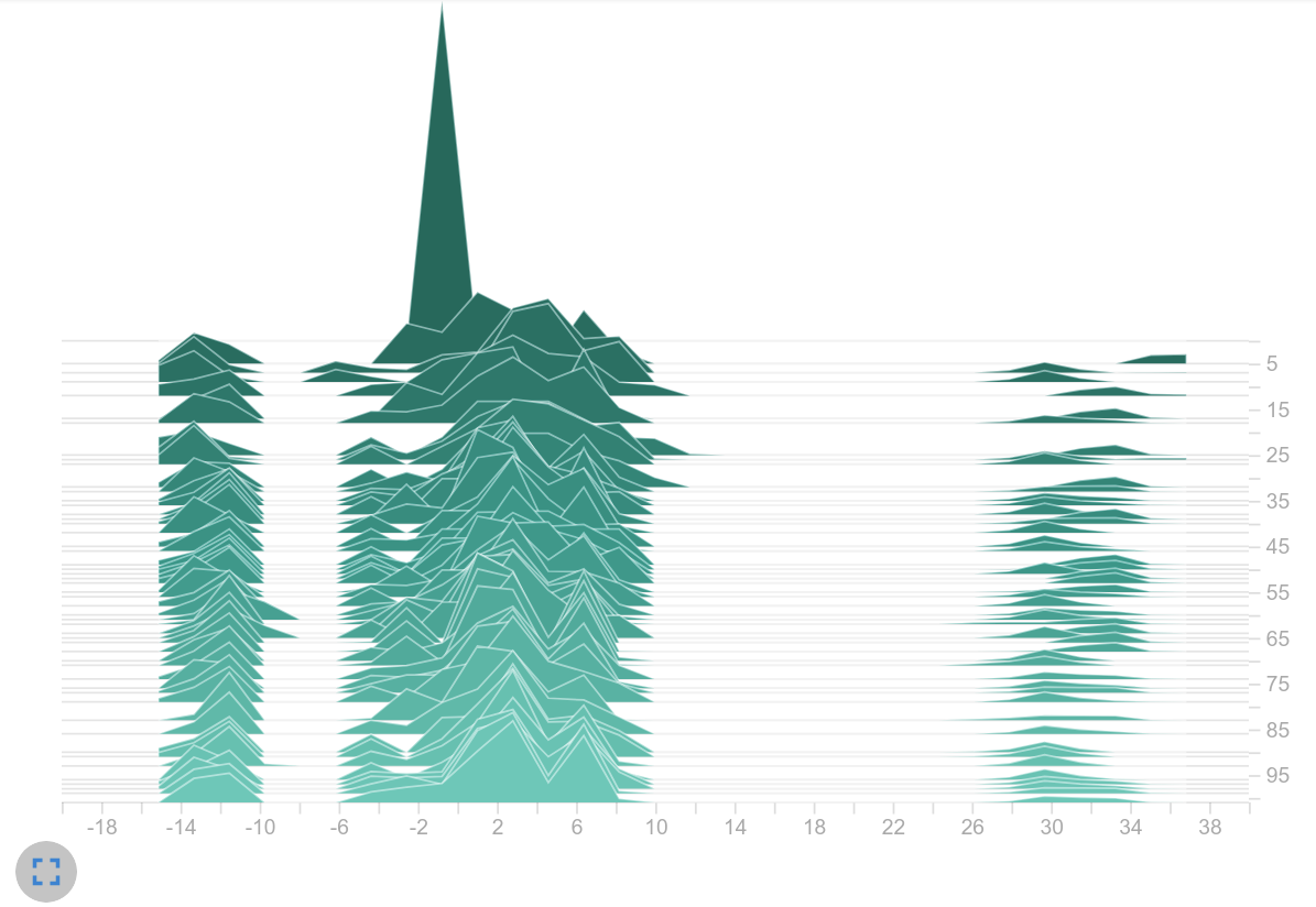
Observation: Because no activation function is applied to the output of the actor and critic, the logits are not limited to an interval. It is noticeable that the logits in the right histogram take up a significantly larger range of values. While in the left histogram it is mainly logits in $[-1, 1]$ , on the right we find values up to $>30$ . Thats a huge difference! Seems like we are on the right track.
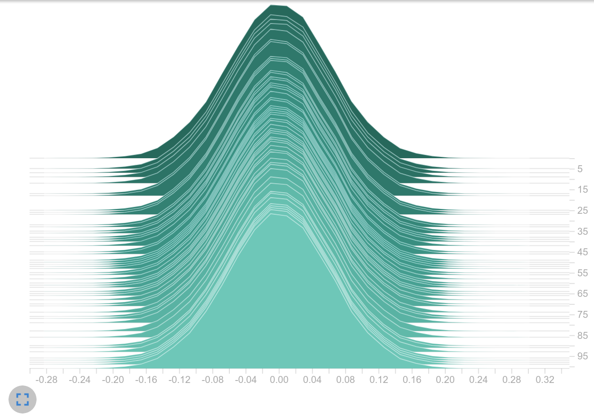
Is one action dominating the policy?
Histogram of sampled actions from $\pi$
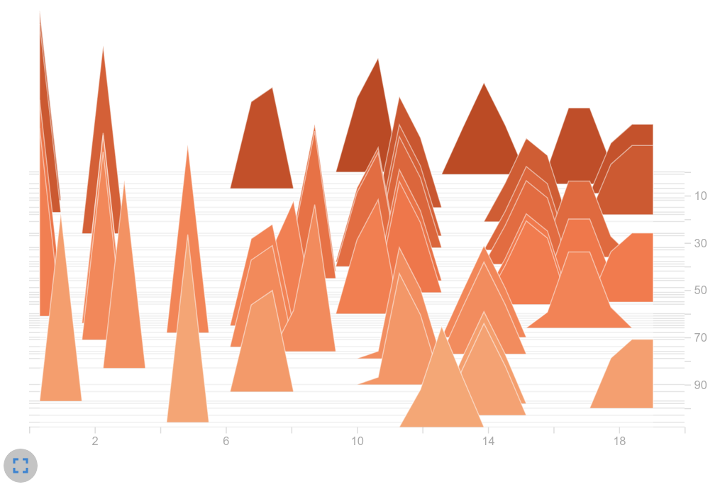
Observation: Our suspicions were confirmed. Our current GCN training led to the same action being selected over and over again. We can clearly see that there is only one peak in the right histogram. In contrast, the baseline shows an expected distribution. Several actions are frequently chosen. So we suspected the big logits as the part of the problem.
Why are there such large logits?: Several reasons came to mind that go hand in hand with the four factors mentioned above:
- The dimension of the latent vector has a direct influence on the magnitude of the logits. Using $d_g = 512$ and $u_g=flatten$ , the latent vector has a length of $512\times23=11776$ (because there are 23 nodes). This huge vector is fed into two fully connected layers - one for the actor and one for the critic. I.e. for one of the 19 actions, the weighted sum over $11776$ is computed. With that massive amount of input neurons, the chance is high that the logits will be large. This assumption fits to the observation that the effect is weakened when using $d_{g}=64$ or $u_g=mean$ - both changes reduce the dimension of the latent vector and thus lower the logits (see next figure on the left).
- It is obvious that if this long latent vector also holds big values, you get even larger logits. For each node, $22$ edges are relevant. When using $u_f=sum$ , they are summed up to one feature vector. Thereby the chance is high that there might be a lot of values inside the saturation area of tanh. We can solve this by averaging the $22$ edge-related feature vectors (see the logits on the right).
Policy values (logits)
- As mentioned above, the latent vector contained many values close to either $-1$ and $1$ . This was mainly caused by an unfavorable learning rate and initialization of the weights. Let’s have a look at two weight histograms. The left plot shows the weights $w_f$ that are used for the $f$ - operation. The right plot shows the fully connected layer weights $w_a$ of the actor. In our opinion, the histogram show quite large values for neural weights.
Histogram of weights
The next logical step was to initialize the weights with smaller values, but after an update step we found weight values in a similar range again. This suggests that the learning rate was too high. This assumption might be confirmed as a smaller learning rate led to smaller logits (next plot on the left). It may also be that the magnitude of the gradients themselves is causing the large weight updates. It may be that the use of the sum as aggregation leads to the exploding gradient effect, as it is also mentioned in this article[8].
- Considering the activation function: Using tanh might have a negative influence on the problem because it limits the value inside our network. Since most of the values are in the saturation range, it can be assumed that the changes within the vectors are small for different observations. Since different observations could result in a similar latent vector, only one action is preferred. Removing the upper limit by using relu instead of tanh seemed to solve the issue as well (see logits on the right). However, to us it’s still a mystery why the initially large logits can be lowered when applying relu. It might be because all negative values in the latent vector are clipped to zero and therefore fewer elements are included in the weighted sum within the actor than when tanh is used.
Policy values (logits)
We are not entirely sure why increasing the entropy coefficient did not help to solve the problem. However, we’ve come to the following conclusions:
- With the magnitude of the logits, one may have to increase the entropy coefficient stronger (not just by a factor of 10) until an improvement can occur.
- When attempting to distribute the action probabilities more uniformly, the incorrect size of the learning rate and/or gradients again resulted in large logits, making it impossible for the algorithm to increase the entropy.
Why could big values in $\pi$ be dangerous?
Remember how actions are sampled? Because we’re using a policy-based method, we sample directly from the learned policy. As a reminder, here is the code how actions will be chosen:
def sample(logits):
    noise = tf.random_uniform(tf.shape(logits))
    return tf.argmax(logits - tf.log(-tf.log(noise)), 1)
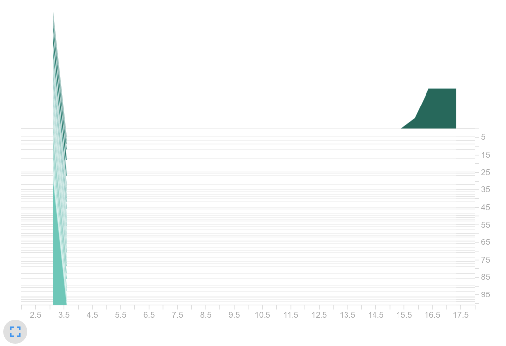
We use the logits to derive actions. We (wrongly) assumed that this kind of sampling requires the logits and noise to be of a similar order of magnitude. Why? Let’s have a look at the histogram of $5000$ Gumbel noise samples (figure on the right):
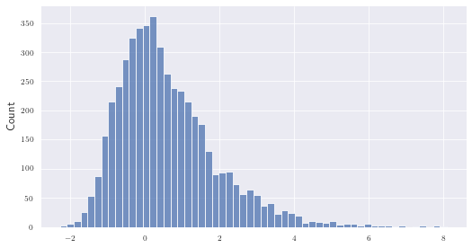
Most values lay in $[-2, 2]$ . Our assumption was that large logits prevent correct action sampling because the noise loses its influence - i.e. only the action with the highest logit would be sampled. Suppose we have five actions and a significantly larger logit for action three: $logits=[-0.2, 0.1, 5, 0.2, 0.3]$ . With most of the noise distributed in [-2, 2] it is very unlikely that any action other than the third one would be chosen.
However, contrary to our assumption, the action sampling process does nothing wrong here! If we would apply a softmax on our logits and interpret the results as probabilities, we would expect the same to happen: $[0.005, 0.007, 0.971, 0.008, 0.009]$ . Therefore, with a probability of $97\%$ , action three is almost always chosen. It’s still seems like a bit of magic that adding a noise to the logits works like sampling from the distribution created by applying softmax (please find the mathematical proof of that in [17]). So the problem is very likely be caused by the fact that we are working directly on the unscaled logits. Nevertheless,
☝️ pay attention to the magnitude of the logits when using policy-based methods.
We’ve explored the cause of the falling entropy problem and presented several possible solutions. For the following experiments we’ve decided to keep the logits small by using $u_f=mean$ , i.e. instead of summing up the outputs of $f$ , a mean operation is applied. Another approach would be to use $u_f=sum$ and apply a $log$ to its output. The logits would still scale with the number of edges, i.e. with the input dimension of $u_f$ , but at least logarithmically instead of linearly.
The decision to use $u_f = mean$ was motivated by the fact that we wanted to continue using $u_g=flatten$ and didn’t want to slow down the training unnecessarily with a smaller learning rate. Likewise, we kept the tanh activation function to remain comparable to the baseline. We wanted to deviate as little as possible from the baseline so that the improvements achieved were actually due to the graph structure and not to modified hyperparameters.
5.5 Solving Entropy Problems
This experiment was used to confirm that using $u_f=mean$ solves the falling entropy problem that we encountered.
Hyperparameters:
- $\mathcal{T}=gcn_{full}$
- $d_{f,g} = 512$
- $u_f=mean$
- $u_g=flatten$
- $\phi=tanh$
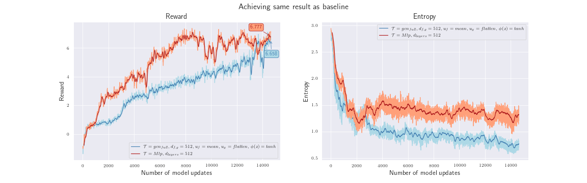
With these results, we think we can confirm $H_3$ , because increasing the number of neurons as well as setting $u_f=mean$ improved the performance. With a similarly good reward compared to the baseline, this was the best result at the time! In our opinion, the entropy curve now shows a valid progression, as we would expect it to.
5.6 Consider Different Edge Types
The next goal is to improve the graph topology. Sometimes we might want to model different types of relationships between different types of nodes. One simple example: The relationship of one football player to another is quite different from that of a player to the ball. To reflect multiple edge types, one may add edge-specific parameters. Instead of one single function $f$ with a specific set of parameters $w_f$ , there are multiple functions, depending on the number of relationships that exists: $w_{f_0}, w_{f_1}, ...$
Why do we want to add this complexity? If all nodes are equal, the ball needs to have the same features as any player, and vice versa, because they are both passed to the same $f$ . This is against our initial idea of logical separation, because then the node $n_{ball}$ has to include player-only features that never apply to it (like yellow card or exhaustion factor). A player would also have to include ball-only features like (rotation values, z position etc.). Having separate edge types for ball-nodes and player-nodes solves this problem.
NB: Technically this creates four different edge types:
| $n_{player} \rightarrow n_{player}$ , | $n_{ball} \rightarrow n_{player}$ |
| $n_{player} \rightarrow n_{ball}$ , | $n_{ball} \rightarrow n_{ball}$ |
A parameterized ball-to-ball connection can’t occur with only one ball in the game. However, we also decided to eliminate the player-to-ball connection type, since the ball is passive and never controlled directly. To do this we slightly altered the graph topology: We no longer update the ball node with new information. Now the two cases in the bottom row never occur and we can ignore them. That leaves us with $k=2$ separate edge types.

Each node type now only contains information relevant to it, that is $16$
ball features and $39$
player features (down from $43$
features for every node).
Since we now have two edge types, we also have two edge functions, $f_0$
(player-to-player) and $f_1$
(ball-to-player) and two subsets of edge representations $\tilde{E}_0$
and $\tilde{E}_1$
.
Function $g$ now receives three inputs: The node’s original representation, the combined outputs of $f_0$ and the combined outputs of $f_1$ .
Creating a separate feature vector for the ball and the player and thereby creating two edge types, might reflect the ball's special properties better and is more in line with the idea of a graph that encodes information. Also, deleting edges that flow into the ball should not affect performance as the ball is treated as an independent object that does not need information about the players around it.
$\mathcal {H_4}$ = The separation of ball and player nodes enables a better flow of information and thus increases the overall reward.
$\mathcal {H_5}$ = Deleting player-to-ball edges should not have a negative effect.
Since for each node only one output of $f_2$ is relevant (the edge that comes from the ball), there is no need to apply $u_f$ on the results of $f_2$ .
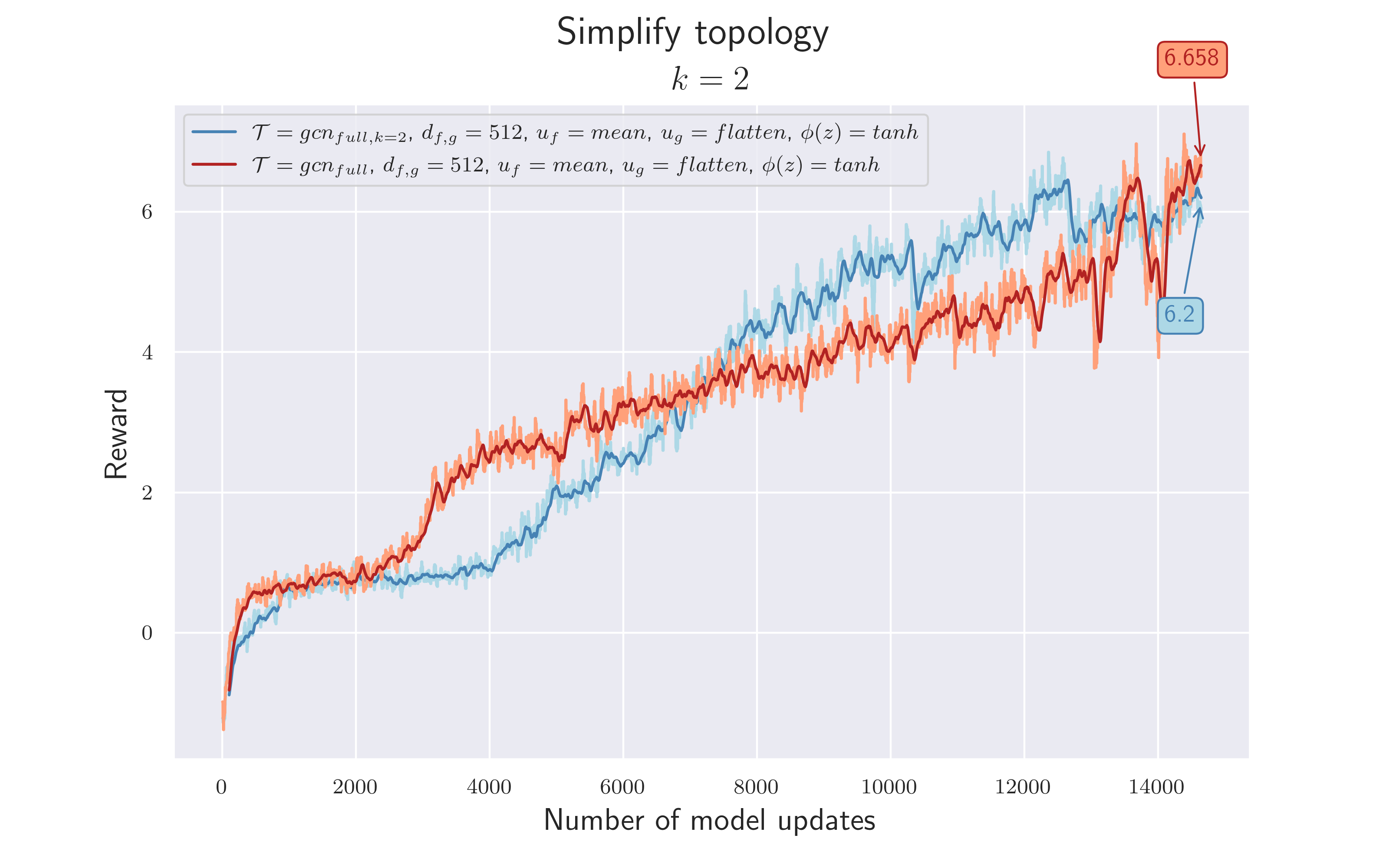
Results are compared with 4.5. There is no great difference in the total rewards. What's noticeable is that a reward $>6$ is reached more quickly. However, we can assume a similar model quality, since the training variance is within a typical range. This seems to confirm $\mathcal {H_5}$ , but not $\mathcal {H_4}$ as no decisive advantage could be observed. Perhaps the complexity of all players being connected to all other players was still too great to see any improvement in the current training time.
5.7 Introduce Star Topology to Reduce Noise
So far our topologies $\mathcal T$ have been (mostly) fully meshed. Every node (except for the ball in 4.6) receives information about every other node. This is a somewhat naive approach, because it assumes that all nodes are created equal, and all neighboring nodes may carry important information in any given game state.
We now consider an alternative topology, a star. This topology sees the active player in the center, with all surrounding nodes (players and ball) only feeding their information into it. These other nodes still feed their own information back to themselves, but don’t have any incoming edges. This decision seems sensible, since the action sampled by the agent will only be executed by the active player. Updating the information of the surrounding players isn’t expected to improve their representation, but might even lower their signal to noise ratio with redundant information.

We now drastically reduced the complexity of the topology by using a star topology. Whereas the fully-meshed version contains $506$ edges, the star topology reduces the number to only $22$ .
It is sufficient to consider only the active player, since only this player provides the possibility to interact with the environment. Updating the representation of the active player by considering its $21$ connections is sufficient. The output of the GCN is now $=h^{n_{act}}_1$ .
$\mathcal {H_6}$ = The use of star topology reduces the environment’s complexity without compromising performance.
$\mathcal {H_7}$ = Since the complexity of the topology is reduced, we can also reduce the complexity of the neural networks by using $d_{f,g}=64$ again, without degrading performance.
In order to implement the star topology, all edges that do not flow into the active player node are omitted. Now, the function $u_g$ is considered as a filter function that simply returns the updated features of the active player node and discards everything else. Since these experiments aren't presented in chronological order, this experiment assumes $k=1$ , therefore using the same features for ball and players. We stick to $u_f =mean$ and a $tanh$ activation.
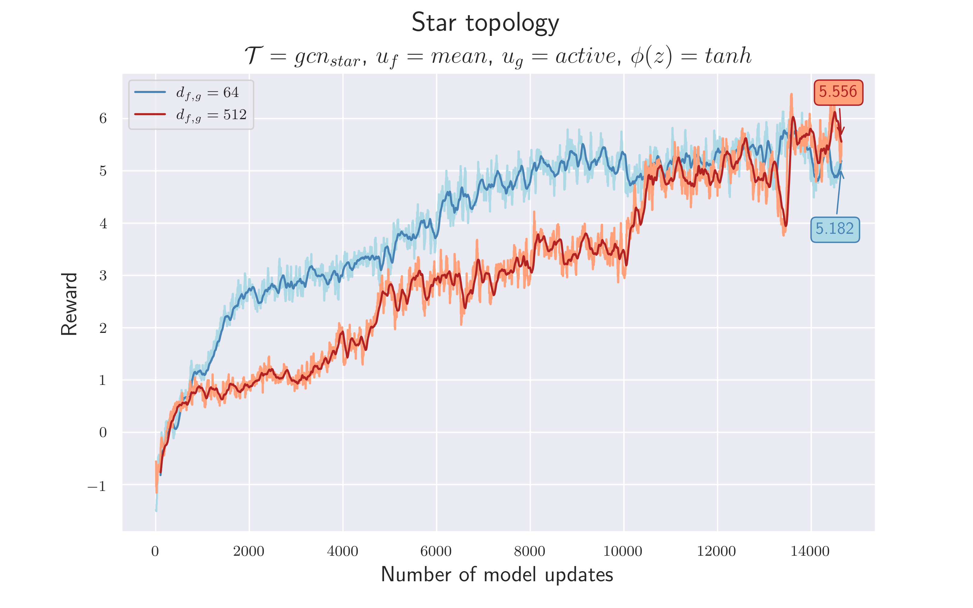
We consider both hypotheses to be confirmed, as the differences to previous results are only slightly smaller. This could also be due to an unfavorable end of training, as values $>6$ were achieved shortly before. Although we now had a much more dynamic topology, it worked!
5.8 Use Previous Concepts and Introduce Globals
Since we still think it makes sense to use different edge types, we transferred the concept of using $k=2$ to the star topology, separating features per node type again.
In addition to the node-specific features, there are actually some global features that do not belong to either a player or the ball (current game mode, sticky actions etc.). If we use a pure GCN structure, that information has to be routed through the nodes, adding redundance and causing larger node state vectors. Instead, we tried bypassing the GCN with the global features, and simply appending them onto $input_{actor, critic}$ . This introduces $17$ global features and reduces the node-specific ones down to $9$ ball features and $20$ player features.

The separate consideration of the ball and the players should enable the algorithm to better process the ball information. Moreover, by excluding the globals from the GCN process, we include more domain knowledge.
$\mathcal {H_8}$ = We can improve the star topology by using two edge types and “skip-connections” for the global features.
The idea of using $k=2$ is the same as in 4.6. Also, features that are considered global are now wrapped around the graph and merged with its output. We keep the so far best hyperparameters and train with $d_{f,g}=512$ and $d_{f,g}=64$ .
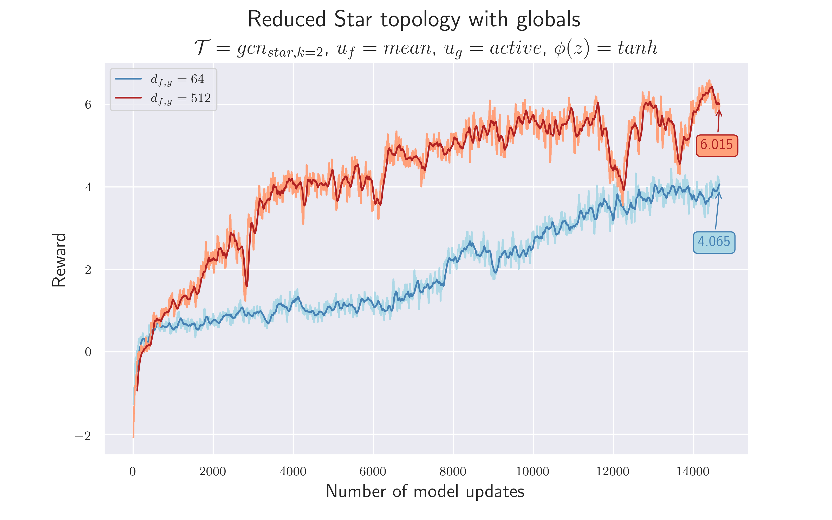
It is difficult to make a clear statement about the validity of $\mathcal {H_8}$ based on these results. On the one hand, compared to the previous star topology, there is a clear improvement when using $d_{f,g} = 512.$ The total reward and the training speed is higher ⇒ a reward of $4$ is achieved after less than half as many model updates. On the other hand, the introduced changes seem to have a negative effect when using $d_{f,g}=64$ . This may be caused by the globals and the output of $g$ not being scaled to the same statistics. The globals are considered to be discrete, one-hot encoded variables - they are either $0$ or $1$ . The output of $g$ is something real-valued and is pushed into $[-1, 1]$ by the $tanh$ . This might lead to the fact that their information is not weighted with equal importance, and thus valuable information is lost. We may explore better scaling options in the future.
5.9 Final Experiment: Reduce Neighborhood
Since the previous approach worked in principle, we wanted to simplify the topology further.
Because let’s be honest: Does the active player really need the information of all other players at all times?
Especially if the goal is to solve the problem of playing football and not to learn complex strategies (which is difficult anyway when controlling only one player), it may not be necessary to use the information about every player at every moment. The more we sensibly reduce the complexity of the graph, the easier it is for the algorithm to learn how to solve the given task. Another perspective may be that the ball information is still drowned out in the "noise" of the $21$ player edges. Reducing their number, e.g. down to $5$ players per team, could drastically reduce such noise.
$\mathcal {H_9}$ = Information of the ball node, as well as those nodes closer to the active player, is more important than that of players further away. This allows the player nodes that are not near the active player to be left out without negative consequences.
To verify the hypothesis we only consider the five nearest players from each team. We use a euclidean metric to measure distance. Hyperparameters as in 4.8 are used.
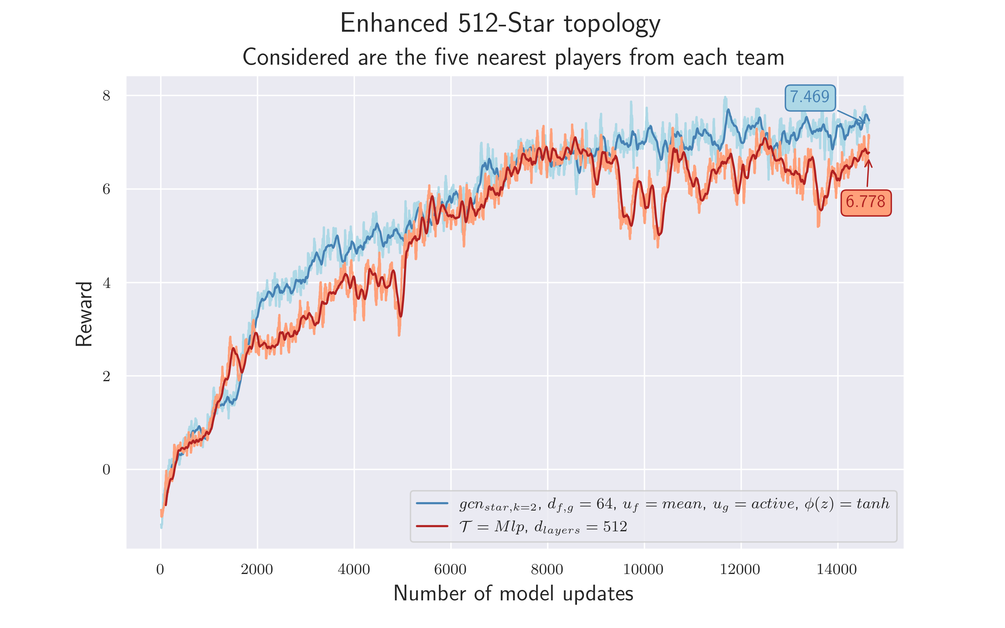
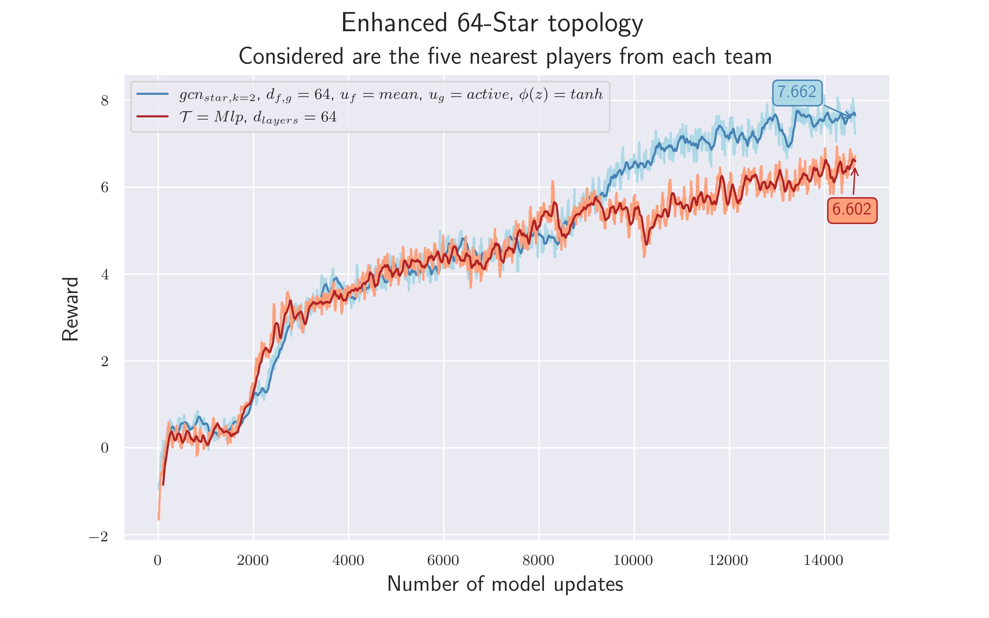
Isn't it nice when the last experiment leads to the best result?! As both results show, omitting distant players does not lead to a loss of important information - $\mathcal {H_9}$ confirmed. On the contrary, it seems easier for the model to find a strategy to solve the task - both training runs achieved a total reward $>7$ , new personal record! 😏 Ah well. If only the semester was longer.
6. Conclusion
Great to see you’ve made it down here! After our journey through all those experiments, it’s time for a conclusion.
What about $\mathcal {H}$ ?: We did need quite a lot of experimentation before we even achieved performance comparable to the MLP. While the last two results could technically lead us to consider $\mathcal {H}$ confirmed, neither of us feel completely confident to do so. The GCN’s performance lead isn’t huge, which makes it very hard for us to say that GCN are definitely better at the task. Although we achieve a slightly higher total reward at the same speed, the complexity of the architectures isn’t entirely comparable, and getting a robust validation of our results is computationally impractical.
Is a GNN really suitable for this kind of task? At this first glance we got, it looks promising. But we cannot say that with certainty, because of the following reasons:
- In this scenario, the graph is small but the topology is dynamic (at least when using a star topology). In many GNN-scenarios, the graph is very large, but the topology is fixed.
- A true test of GNN with reinforcement learning might require both a large graph and a dynamic environment. Realtime strategy games might be a good option for this.
- Advantages and disadvantages of a GNN may only appear after longer training, with more diverse opponents - or not at all if the use case doesn’t fit.
- A final mean reward of around $\sim7$ might the best possible result, given the simple numerical observations. Further improvements might be only possible through additional features (e.g. hand-crafted, temporal etc.) and more suitable topologies (see Future Work).
That said, we are still really satisfied with the results: We’ve combined graph neural networks and reinforcement learning, and we even (eventually) achieved one of our main goals - a higher average reward than the MLP baseline. For a total shot in the dark, we would say this is a great success!
Future Work
All things considered, it does look like we are on the right track. More experiments are definitely needed, and we have plenty of ideas yet to try:
Different training setup: Of course, it is always possible that any decisive advantage will only become apparent with longer training or with a different training setup. Our current resource limitations make this unlikely to happen.
Encode more domain knowledge into $\mathcal{T}$ : Our biggest jump in performance occurred after changing the topology to filter out over half the players. The existing edges in a graph only tell half the story: It might be equally important to consider which edges aren’t there. We’ve only tried simple topologies so far, i.e. fully meshed and star, and we only filter player nodes by proximity to the active one. But there is practically no limit to the information we could encode. We might do such things as:
- Limit the number of nodes connected to the active player to three per team. Keep in mind that this may prevent the model from learning more complex strategies (like a high pass from defender to striker).
- Use a player’s role to filter which players are more important to the active one.
- Hardcode “known” player constellations and filter nodes based on them.
- Allow for a different number of nodes at each state, to enable more complex logic. GCN can generally support this (shared weights).
Use a deeper architecture: So far, we only use a single GCN layer. You probably wouldn’t use a CNN with a $3\times3$
receptive field on a $3\times3$
image, either. It isn’t entirely comparable, because we still have the added complexity of the $f$
and $g$
functions, but there is likely some functionality lost, that might be useful.
However, we are critical of this idea, as we would have to filter player nodes out first, only to give that information back through message passing, anyway.
Besides, the two main advantages we expect from the GCN are that we can leverage variable node counts and graph-encoded domain knowledge, which both don’t necessarily require a deeper architecture.
Model an entirely different GNN architecture: Out of the possible advantages of GCN that we projected earlier, the only one that really made a difference for us was the direct application of domain knowledge, by encoding it into the graph directly. This concept could go even further, by choosing a better-suited GNN architecture. We have only begun to understand GNN and what is possible with them, so our own GCN architecture is a very simple one. However, the following concepts could prove useful:
-
We could not only assign a feature vector to each node, but also use edge features. As such features the distance and angle would be conceivable, since these two define the vectors of the players relative to each other. Have a look at Exploiting Edge Features in Graph Neural Networks and Dynamic Edge-Conditioned Filters in Convolutional Neural Networks on Graphs that introduce edge features in graph neural networks in general.
-
In CNNs, we often find the concept of pooling to reduce computational costs and memory requirements. For a future deeper GNN architecture it may be a good idea to adopt this concept, as done in Pooling in Graph Convolutional Neural Networks, to reduce the number of learned parameters and to control overfitting.
-
So far, all edges flow equally into the combination (or aggregation) functions. Of course, this is not ideal because the importance of edges may vary. To let the model learn which part of the data is more important than others, we could apply the concept of attention to graph neural networks and assign different weights to different nodes in a neighborhood. A good starting point would probably be Graph Attention Networks.
-
In football, actions are significantly influenced by previous actions. Modeling long-term dependencies could therefore improve the game in any case. Within the GFootball context, we’ve observed three ways to include temporal information:
- the direction vectors inside the raw observations,
- stacked image representations and
- an LSTM layer after the feature extractor.
Now that we have modeled the dependencies between players, it would be intuitive to use temporal information within the graph. Gated Graph Recurrent Neural Networks might be useful for that since they take both the temporal and graph structures of a graph process into account.
6. Sources
[1] https://www.kaggle.com/c/google-football
[2] Online-Erfahrungsbericht Kaggle
[3] https://arxiv.org/pdf/2006.12576.pdf
[4] https://gym.openai.com
[5] https://github.com/google-research/football/tree/master/gfootball/doc
[6] https://github.com/BazkieBumpercar/GameplayFootball
[7] https://towardsdatascience.com/a-gentle-introduction-to-graph-neural-network-basics
[8] https://ai.plainenglish.io/graph-convolutional-networks-gcn
[9] https://tkipf.github.io/graph-convolutional-networks/
[10] https://www.microsoft.com/en-us/research/video/msr-cambridge-lecture-an-introduction-to-graph-neural-networks
[11] https://deepmind.com/learning-resources/-introduction-reinforcement-learning-david-silver
[12] http://www.incompleteideas.net/book/RLbook2020.pdf
[13] https://github.com/openai/baselines
[14] https://www.davidsilver.uk/wp-content/uploads/2020/03/pg.pdf
[15] https://arxiv.org/pdf/1907.11180.pdf
[16] https://arxiv.org/abs/1707.06347
[17] https://lips.cs.princeton.edu/the-gumbel-max-trick-for-discrete-distributions/
7. Notation
- $\mathcal{T}$ ⇒ Topology of the underlying feature extraction network. Basic distinction is made between MLP (baseline), $gcn_{full}$ and $gcn_{star}$
- $G$ ⇒ Graph of vertices (nodes) $V$ and edges $E$
- $V$ ⇒ Set of all vertices (nodes) $n$
- $H$ ⇒ GCN hidden state, set of all node states $h^n$
- $H_0$ ⇒ Input data $X$ for the GCN
- $E$ ⇒ Set of all edges
- $\tilde{E}$ ⇒ Set of all edge representations $e$ in a GNN layer
- $\phi$ ⇒ Activation function applied on every layer output of the MLP and on the $g$ and $f$ operation inside GCN topology
- $d$ ⇒ Dimensionality, i.e. the number of neurons used for the layers or as output of the $g$ and $f$ operation inside GCN topology
- $f, g$ ⇒ Two separate neuronal networks. $f$ receives target and source node state and computes an edge-related feature vector. $g$ reiceves the target state and the aggregated edge-related feature vectors and computes the updated node-state
- $w_f, w_g, w_a$ ⇒ Trainable parameters of $f$ , $g$ and actor.
- $u_f$ ⇒ Node-wise commutative combination of the outputs of the $f$ -operation are commutatively combined per node.
- $u_g$ ⇒ Global commutative combination of hidden state $H$ , output is passed to actor and critic
- $k$ ⇒ Number of edge types.
- $h^n_{t-1}$ ⇒ State of the node $n$ at layer $t-1$ .
- $i, j$ Indices for nodes $n_i,n_j\in V$ and corresponding edge states $e_{ij}$ in $\tilde{E}$