

Selected Topics #2:
3D Ken Burns Effect from a Single Image
Download the tutorial as jupyter notebooks
Table of Content
- 1. Introduction
- 2. Architecture
- 3 Training the Networks
- 4. Results
- 5. Problems
- 6. Demo
- 7. References
1. Introduction
The introduction will begin with the explanation of the 3D Ken Burns Effect. We will elaborate what this effect is and how it works but also what it takes to create it based on just one single image. After that, the paper is presented, which was the basis and motivation for this notebook. Last but not least we will talk more about the training data that is needed and that we used in order to create the 3D Ken Burns Effect from a Single Image.
A live demo of the 3D Ken Burns Effect is provided to create your own effects from a single image of your choice. It can be found in section 6. Demo.
1.1 3D Ken Burns Effect
The Ken Burns Effect is a technique used to animate a still image by panning and zooming through the image (Fig. 1). Another variation of this effect is called the 3D Ken Burns Effect (Fig. 2), which is achieved by adding parallax effects to the individual objects in the scene.
The 3D Ken Burns Effect yields a more immersive experience for the following reasons:
- The positions of the objects in the image change while the panning effect is applied.
- The sizes of the objects in the image change while the zooming effect is applied.
Since the objects’ positions and sizes depend on the panning or respectively the zoom, creating the 3D effect manually is a time and labour-intensive task, including the following steps:
- Mask and cut out all objects into separate layers. (Fig. 3)
- Adjust every objects’ positions and sizes according to the panning and zoom setting for N frames. (Fig. 4)
- Inpaint occluded areas with a graphics editor. (Fig. 5)
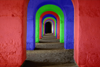
Fig. 3: Masking and cutting objects
Fig. 4: Adjusting objects’ positions and sizes
Fig. 5: Inpainting occluded areas
The objective of this work is to create a 3D Ken Burns Effect from a single image without depth information. Since depth information is crucial for generating this effect, it needs to be estimated from the input image. For this reason a Depth Estimation pipeline is responsible for estimating, adjusting, and refining the depth map. A point cloud is then generated from the input image and its depth map by a View Synthesis pipeline. The point cloud is a 3d representation of the still image and its depth map. Since there are missing information in the 3d scene through occlusion, these areas needs to be inpainted with regard to color and depth values. The View Synthesis pipeline is responsible for extending the point cloud until occluded areas are filled with color and depth information. The 3D Ken Burns Effect can than be generated by moving a camera through the extended point cloud and capturing a sequence of images. These images are then combined to create a video of the 3d effect, which can be seen in Fig. 6.
1.2 Reference Paper
The main inspiration and basis for this notebook has been the paper “3D Ken Burns Effect from a Single Image” by Simon Niklaus (Portland State University), Long Mai (Adobe Research), Jimei Yang (Adobe Research) and Feng Liu (Portland State University), published on the 12th of September, 2019 [1].
Niklaus and Liu, his professor at Portland University, have furthermore published and worked on various other papers in the area of image and video editing, segmentation and augmentation through deep neural networks.
Luckily, most of the code - except for the implementation of the trainings for the different networks - as well as their specially created training data has been made available for the public, which enabled the work in this notebook (see here) The training data will be more thoroughly covered in the following section.
1.3 Training Data
In order to estimate a depth map from a single image, depth information need to be presented while training the depth estimation model. For this reason, Niklaus et al. provided a synthetic dataset, which includes indoor scenes, urban scenes, rural scenes, and nature scenes. Fig. 7 displays some of the available environments.
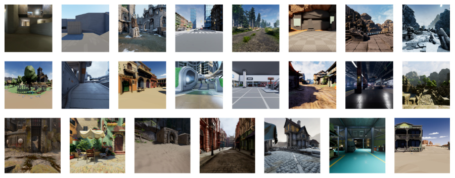
Fig. 7: Synthetic dataset consisting of 32 virtual environments
The synthetic dataset consists of computer-generated images from 32 virtual environments. From each image sample an accurate ground truth depth map can be extracted, which can be seen in Fig. 9. Each image and depth map has a resolution of 512 x 512 pixels. The images were captured by a virtual camera rig moving through each virtual environment in two different modes as depicted in Fig. 8. First the camera flies through the scene to capture samples. Secondly the camera walks through the scene, which allows to capture samples from an angle humans would receive. The different capture modes add variance with regard to angles. This variance will be useful to train a more generalizing model, which is capable to estimate depth maps from images with different angles. As shown in Fig. 9 each sample consists of 4 different views. This is done to augment the dataset with more images.
Each captured view contains the sample which is shifted in 4 directions:
- top left
- top right
- bottom left
- bottom right
The synthetic dataset contains of 76048 unique samples, where each sample consists of 4 shifted views. Thus resulting in a total of 304192 images and depth maps are available for the training.
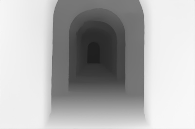
For each image a corresponding depth map is provided, in order to be able to learn and predict a depth map from a 2d image (Fig. 9). This depth map contains a 16 bit value for each pixel in the range of $0$ and $2^{16}-1=65535$ . Pixels which appear near are assigned a values close to $65525$ , whereas farther pixel have values close to $0$ . Estimating an accurate depth map is crucial for generating the 3D Ken Burns Effect, since a point cloud will be calculated from the 2d image and its depth map, which will represent the 3d structure of the still image. It is important to conserve the geometrical structures in order to create an immersive 3d effect.
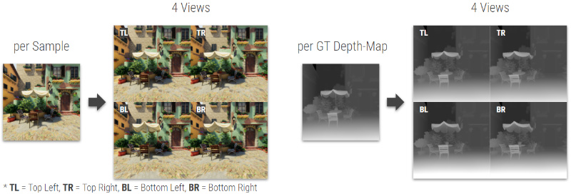
Fig. 9: Synthetic dataset: 4 views for each sample and depth map
2. Architecture
The network architecture for the process of generating the 3D Ken Burns effect from a single image can be divided into two different pipelines. The first pipeline is the so called Depth Estimation Pipeline, which, as the name implies, ultimately provides a depth estimation based on our single image input. With this depth estimation, the second pipeline comes into play, the View-Synthesis Pipeline. This pipeline will take the depth information as well as the original image in order to provide a point cloud. The resulting point cloud can then be used to create the 3D Ken Burns effect for any given start and end point.
The two pipelines will be separately examined in more detail in the following sections.
2.1 Depth Estimation Pipeline
The Depth Estimation Pipeline represents the starting point of the network. It is more specifically a Semantic-aware Depth Estimation Pipeline, meaning that it estimates the depth of its input image in a way that it can detect and optimize semantically important or respectively related areas of the image. This semantic addition is necessary in order to tackle three key problems that occur when applying existing depth estimation methods to generate the 3D Ken Burns Effect. Niklaus et al. discovered these problems during their work and they will be further examined now.
1. Problem: Geometric distortions
Existing depth estimation methods like MegaDepth [2] do a good job in generating depth orderings, but a big problem when trying to generate the 3D Ken Burns with their depth estimation is the lack of awareness for geometric relations such as planarity. This often leads to geometric distortions, as we can observe in the image above. When moving the camera from side to side, undesirable bending planes appear in the view synthesis result.
2. Problem: Semantic distortions
Another major problem of existing depth estimation methods is the missing consideration of semantic relations. As the above image shows, differing depth values have been assigned to different body parts (body, head, hand) of the child when using MegaDepth [2]. This falsely leads to the child being torn apart when moving the camera.
3. Problem: Inaccurate depth boundaries
The last big issue of existing depth estimation methods is the fact that they process the input image at a low resolution and eventually use bilinear interpolation to create a depth estimate at full resolution. Therefore, those techniques have problems with capturing depth boundaries. This lack of accuracy mostly results in artifacts when trying to render novel views.
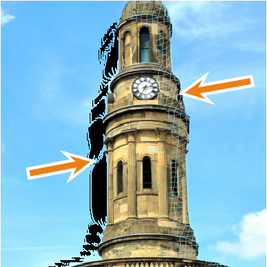
Fig. 12: Inaccurate depth boundaries
The Depth Estimation Pipeline itself can again be divided into three main parts. Every part respectively tackles one of the key problems stated above. The three parts are the Initial Depth Estimate, the Depth Adjustment and the Depth Refinement. The full pipeline can be seen in the image below and the three parts will subsequently be covered in full detail.
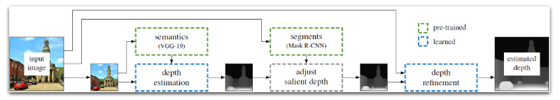
Fig. 13: Depth Estimation Pipeline
2.1.1 Initial Depth Estimation
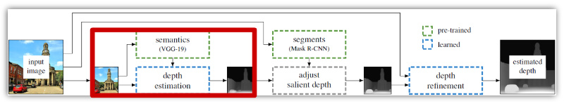
Fig. 14: Initial Depth Estimation (red area)
As can be seen in the image above, the input image is passed through VGG-19, a well known deep neural network for image classification. More specific, the feature maps of the fourth pooling layer of VGG-19 are extracted. The extracted semantic informations about the image are used, besides the image itself, for the initial depth estimation.
For the Initial Depth Estimation, a GridNet architecture has been chosen by Niklaus et al. A GridNet consists of several paths or streams from the input image to the output prediction, which work with different image resolutions. Streams with high image resolutions enable the network to make more accurate predictions, while streams with low resolutions transport more context information thanks to larger receptive fields. The streams are connected by convolutional and deconvolutional units to form the columns of the grid. With these connections, low and high resolution information can be exchanged.
The below image shows a vague representation of the GridNet. The image itself is inserted into the first row of the network, while our previously extracted feature maps from VGG-19 are inserted into the fourth row. Since the channel size for all grid items of the bottom half of the network is significantly bigger than those of the upper half, the network focuses more on the semantic informations than the image itself. Niklaus et al. found out that providing and focusing on this information pushed the network to better detect the geometry of large structures, which was the first key problem that has been examined before.
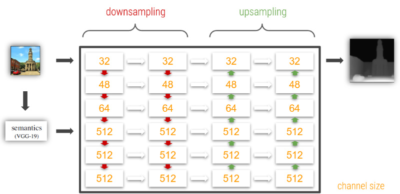
Fig. 15: Coarse representation of the used GridNet architecture
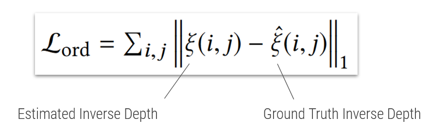
Loss function
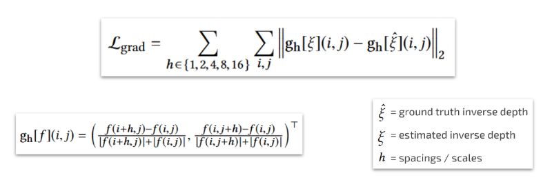
The loss function for this network combines a pixel-wise l1-based loss with a scale invariant gradient loss, whereas the emphasis is on the scale invariant gradient loss.
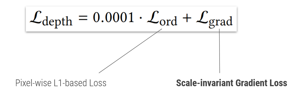
The pixel-wise loss basically compares every pixel of the Estimated Inverse Depth with the corresponding pixel of the Ground Truth Inverse Depth and computes the sum of the differences between all of them. Niklaus et al. found this loss alone to be insufficient for the given task and decided to add another loss.
The scale invariant gradient loss, which was then added, has been proposed by Ummenhofer et al. [3] in order to encourage more accurate depth boundaries and also stimulate smoothness in homogeneous regions. It does so by not only comparing the difference between two pixels, but also factoring in neighboring horizontal and vertical pixel areas. This means that for every viewed pixel, the computed loss is not only the difference between its value and the value of the representative pixel in the ground truth image, but also neighboring pixels are going to be compared and weighted into the computation. This happens multiple times at different scales h for the amount of viewed neighboring pixels. By doing that, the loss also penalizes the relative depth errors between adjacent pixels.
The difference that the addition of this gradient loss brings can be seen in the following image, taken from the original paper by Ummenhofer et al. [3]. We observe that the boundaries of the different objects in the image are more clearly visible when using the combined loss. Furthermore, the depth values for the homogenous region of the matress are way more consistent in the second image (combined loss) compared to the first image (only l1-based loss).
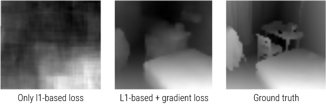
Fig. 16: Loss comparison
Result
After the Initial Depth Estimation, the problem of geometric distortions has successfully been tackled. We can see this when comparing the 3D Ken Burns Effect results, once using the Depth Estimation of MegaDepth and once the Initial Depth Estimation of Niklaus et al.
2.1.2 Depth Adjustment
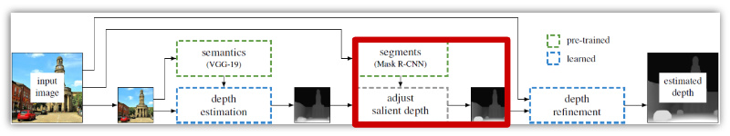
Fig. 18: Depth Adjustment (red area)
The second part of the first pipeline is the Depth Adjustment. The result of this part is an adjusted version of the initial depth estimation, which now ideally has consistent depth values for regions of the same object and therefore tackles the second key problem of semantic distortions.
In order to achieve that, Niklaus et al. make use of Mask R-CNN. Mask R-CNN is a deep neural network that provides high-level segmentation masks for all kinds of objects in an image. For the Depth Adjustment, specifically objects of semantically important objects like for example cars and humans have been extracted by Niklaus et al.
The subsequent process is pretty straightforward. For every extracted mask, take the corresponding area of the initial depth estimate and assign a constant depth value for the whole area. Niklaus et al. state that this approach is not physically correct, but nevertheless produces very plausible results for a wide range of content when applying the 3D Ken Burns Effect.
Result
After the Depth Adjustment, the problem of semantic distortions has successfully been tackled. We can see this when comparing the 3D Ken Burns Effect results, once using the Depth Estimation of MegaDepth and once the Depth Adjustment of Niklaus et al.
2.1.3 Depth Refinement
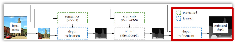
Fig. 20: Depth Refinement (red area)
The last part of our first pipeline is the Depth Refinement. In this part, the so far low-resolution depth estimation is going to be improved and object boundaries will be refined, thus tackling the third and last key problem: Inaccurate depth boundaries.
Niklaus et al. chose a U-Net architecture for this last part. A U-Net architecture is similar to a GridNet architecture in that it has different streams where image informations are processed at different resolutions. The image below shows a coarse representation of the applied U-Net. It gets both the original image as well as our adjusted depth estimation as an input. The adjusted depth estimation is inserted at the bottom of the U-Net. That way, the network learns how to upsample the low-resolution depth estimation with the help of the high-resolution original image, which is both down-/upsampled and kept at the same resolution through the different streams. Because information is shared between the streams, the U-Net is able to produce a refined, high-resolution depth estimation.
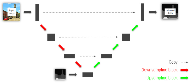
Fig. 21: Coarse representation of the used U-Net architecture
Loss function
The loss function for the Depth Refinement is the same as for the Initial Depth Estimation.
Result
After the Depth Refinement, the problem of inaccurate depth boundaries has successfully been tackled. We can see this when comparing the point cloud rendering results (will be covered in more detail in section 2.2), once using the Initial Depth Estimation of Niklaus et al. and once the Depth Refinement of Niklaus et al.
(a) Using Initial Depth Estimation from Niklaus et al.
(b) Using Initial Depth Estimation from Niklaus et al
2.2 View Synthesis Pipeline
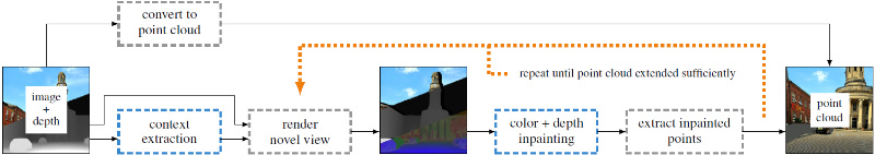
Fig. 23: View synthesis pipeline Source
The overview for the View Synthesis pipeline is illustrated in Fig. 23. The pipeline takes the 2d image and its estimated high resolution depth map, obtained from the Depth Estimation pipeline, as inputs. The output of this pipeline is the point cloud and respectively the extended point cloud, which is created from its input image and depth map. From this point cloud the resulting video frames are synthesized from a moving camera-path. Since the camera captures scenes from different viewing positions, disocclusions will happen. These disocclusions need to be inpainted not only with color values but also depth values. For this reason a context aware color- and depth-inpainting is used to fill in the mission information. The inpainting will be done only in extreme views, specifically in the starting and ending frame of the camera path, to enable real time computation of the 3D Ken Burns Effect. The inpainted pixels will then be added to the existing point cloud, thus extending it with geometrically sound information. From the extended point cloud, a sequence of view renderings will be synthesized, in order to create the video frames for the 3D Ken Burns Effect.
2.2.1 Novel View Synthesis
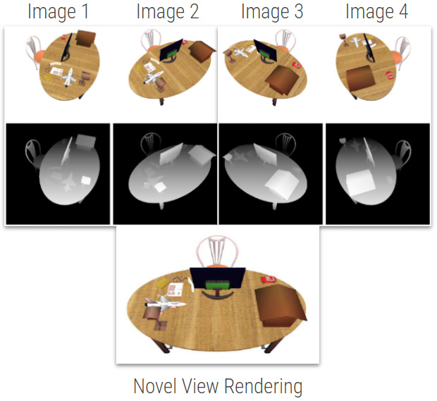
Fig. 24: Novel view synthesis Source
View Synthesis deals with generating new views either from a single image and its depth map, or multiple images from different viewing angles (Fig. 24). In this work both methods are necessary for creating novel view renderings.
First a point cloud will be generated by using the input image and its depth map. The point cloud can be generated by calculating 3d pixels from the images 2d pixels and its’ depth map pixels, which provide information, of how distant the corresponding 2d pixel is from a specific camera position (Fig. 25). From this point cloud new view renderings can be calculated by using planar projection visualized in Fig. 26 and moving the camera along its principal axis while capturing new scenes.
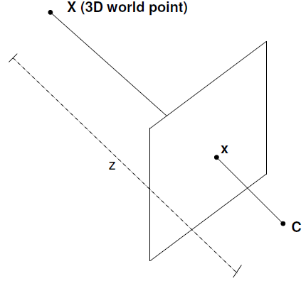
Fig. 25: View synthesis from image and its depth map Source
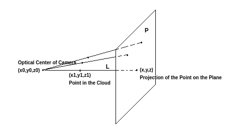
Fig. 26: Creating novel view renderings from a point cloud by using planar projection Source
Secondly novel view renderings from multiple images will be calculated in order to create masked images for the context aware color- and depth- inpainting. For this reason, the synthetic dataset contains 4 views for each captured sample as illustrated in Fig. 9.
The 3D Ken Burns Effect is an extreme form of view synthesis, since from a single 2d image, a high resolution depth map is estimated and used to generate a 3d model. From this point cloud a sequence of novel view rendering are extracted to create the 3D Ken Burns Effect (Fig. 27).
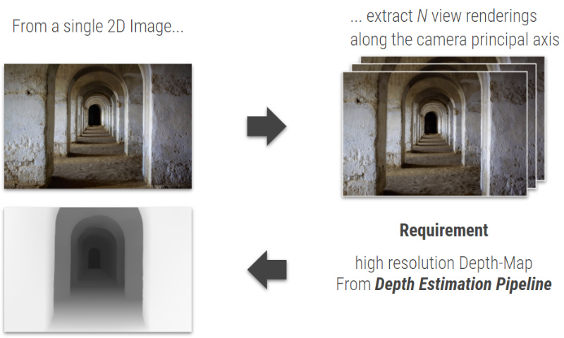
Fig. 27: 3D Ken Burns Effect: extreme form of view synthesis
2.2.2 Creating Point Clouds
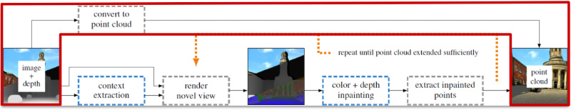
Fig. 28: View synthesis pipeline: creating point cloud
As previously described a point cloud is generated from the input image and its estimated depth map. A resulting point cloud may look like in Fig. 29.
A point cloud can be calculated with the following formula [4]:
$$\mathbf{P}(\mathbf{{x}} ,{z}) =\mathbf{P}( u,v,{z}) =\mathbf{C} +{z} \ \mathbf{M}^{+} \ \mathbf{{x}}$$where:
- $\mathbf{P}(\mathbf{{x}} ,{z})=\mathbf{P}( u,v,{z})$ is a 3d pixel in the point cloud with its 2d coordinates $\mathbf{{x}}= (u,v)$ , and its depth value ${z}$ .
- $\mathbf{C}$ is the camera center in the 3 dimensional space.
- $\mathbf{M}^{+}$ is the pseudo inverse of the calibration matrix, responsible to calculate the camera matrix using extrinsic and intrinsic parameters. The location of the camera in the 3d space is represented by the extrinsic parameters whereas the intrinsic parameters represent the optical center and focal length of the camera.
Fig. 30 describes how a single 3d pixel for a point cloud is calculated. For calculating the whole point cloud, the cameras principle axis has to go through each 2d pixel of the image and placing the 3d pixel in the 3d space depending of its 16 bit depth value. From this point cloud, one can generate as many as possible novel view renderings. however when generating new view renderings, the novel scene has missing information due to disocclusion. These missing information must be inpainted by the context aware color- and depth inpainting method, which Niklaus et al. developed in their paper.
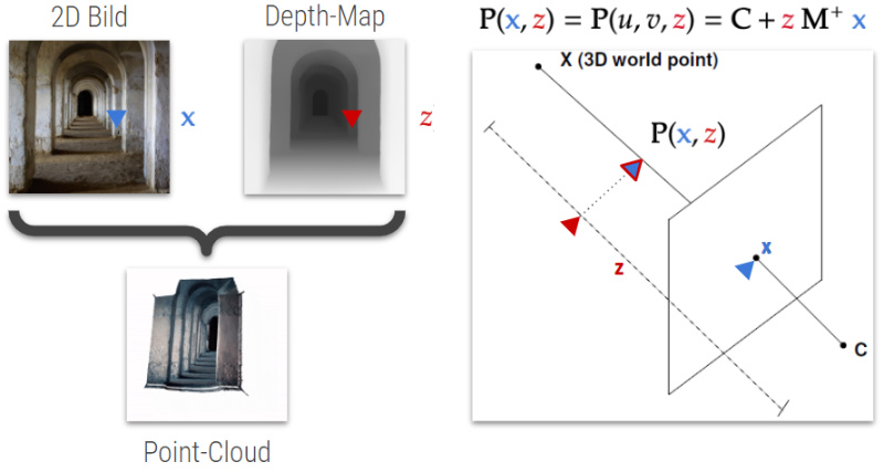
Fig. 30: Point cloud calculation from 2d image and its depth map
2.2.3 Creating context-aware Novel View Renderings
In the previous section we demonstrated how a point cloud can be calculated from a 2d image and its depth map. However we did not explain, how enriching the point cloud with contextual information, is performed to be able to generate high-quality novel view renderings from the enriched point cloud.
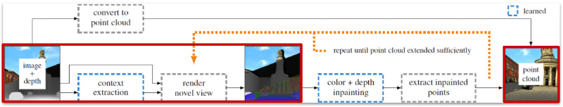
Fig. 31: View synthesis pipeline: creating context-aware view renderings
The contextual information is extracted from the 2d image and its depth map by a separate CNN as shown in Fig. 32. This CNN consists of two convolutional layers followed by a PReLU activation function, which extract 64 channels of context information from the input image and its depth map, which “describes the neighborhood of where the corresponding pixel used to be in the input image” [1]. The context extractor CNN is trained jointly with the color- and depth-inpainting network. This “allows the extractor to learn how to gather information that is useful when inpainting novel view renderings” [1], which are created from the point cloud.
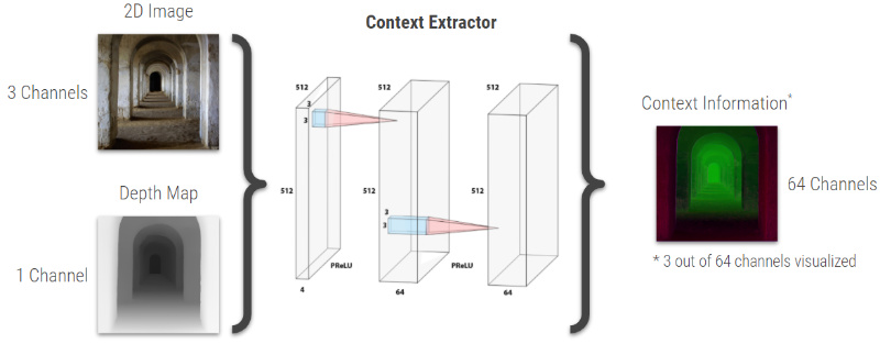
Fig. 32: Context extraction CNN
After the context information is extracted, a point cloud is calculated like demonstrated in Fig. 30. Instead of using only the 2d image and its depth map to create the point cloud, the context information is extended to the 3d pixel (Fig. 33). From this enriched point cloud, one is able to create novel view renderings, which also contain context information.
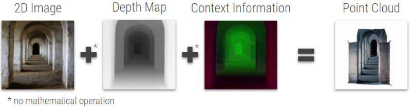
Fig. 33: Creating point cloud from 2d image, its depth map, and context information
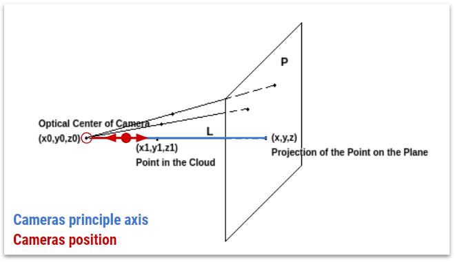
To extract novel view renderings from the context-aware point cloud, one has to project each 3d pixel onto a plane with a certain perspective in the 3d space. Fig. 34 shows how a set of points $(x,y,z)$ can be projected onto a plane $P$ from the optical center of the camera $(x_0,y_0,z_0)$ . The projection $(x,y,z)$ of a point cloud pixel $(x_1,y_1,z_1)$ on the plane $P$ is the intersection between the plane $P$ and a line $L$ passing through the optical center and the point cloud pixel. [5]
The projection onto the plane $P$ is given by the formula:
$Ax+By+Cz=0$
Whereas the line $L$ can be represented as:
$$ \begin{aligned} x = x_{1} + at \\ y = y_{1} + bt \\ z = z_{1} + ct \\ \end{aligned} $$The direction cosines of the line $L$ are $a$ , $b$ , and $c$ . The direction ratio is $t$ . The direction cosines for the lines passing through each projection points $(x,y,z)$ can be calculated if the optical center of a camera, and a set of point cloud pixels are given.
Substituting the equations of line $L$ in the equation of the plane $P$ , yields the point of intersection.
Solving for $t$ results in
$$t=-\frac{Ax_{1} +By_{1} +Cz_{1} +D}{aA+bB+cC}$$The projection of one point $(x,y,z)$ can be calculated by substituting the value $t$ into the equations of line $L$ . For calculating the whole image projection, one has to calculate each projection point like stated before.
Since the 3D Ken Burns Effect needs a sequence of novel view renderings, the calculation of the projection points need to be performed for each single novel view rendering. This is done through moving the camera along its principle axis as seen in Fig. 34. When moving the camera each projection has to be calculated as stated before. With this sequence of images we are ready for filling in the missing information in the view renderings, which are caused by disocclusions.
2.2.4 Color- and Depth Inpainting
After obtaining a sequence of novel view renderings from the point cloud, it is time to inpaint the missing areas with color and depth information.
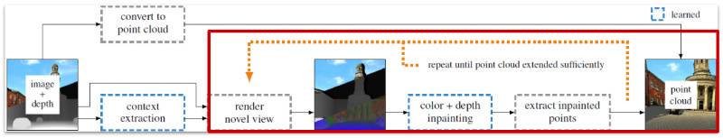
Fig. 35: View synthesis pipeline: color- and depth inpainting
Niklaus et al. implemented an inpainting method which is geometrically and time consistent. In Fig. 36 a comparison between different inpainting methods are compared. The method introduced by Niklaus et al. yields a geometrically and time consistent result as compared to the other methods.
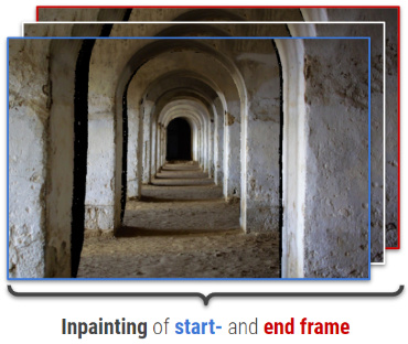
In order to reduce the computation cost of inpainting each view rendering of the sequence, Niklaus et al. decided to only inpaint color- and depth values for extreme viewing points e.g. the start and end frame of the image sequence as visualized in Fig. 37.
After inpainting the start and end frames the inpainted areas are extracted from the view renderings and the new 2d pixels and its depth value will be appended to the existing point cloud. This process is performed like illustrated in Fig. 30, thus extending the point cloud with new information for previously missing areas.
From this extended point cloud, novel view renderings can be obtained by projecting new view renderings from the extended point cloud as demonstrated in Fig. 34. This process of inpainting color- and depth values, extracting the inpainted areas from the view rendering, and extending the point cloud with the inpainted areas is repeated until the point cloud is extended sufficiently.
The 3D Ken Burns Effect can then be generated from the sequence of extended view renderings, by concatenating each individual frame into a video. The whole process is visualized in Fig. 38:
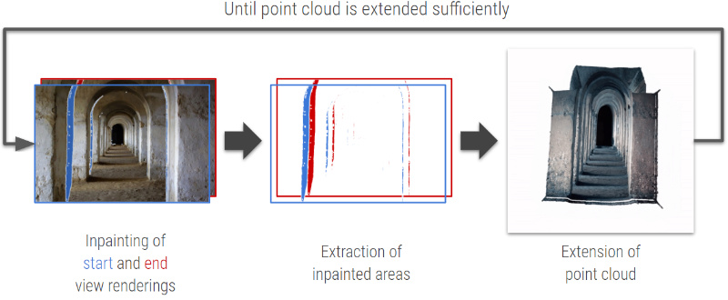
Fig. 38: Point cloud extension
2.2.5 Training Data
Training an inpainting network requires masked images. These masks cover cover some areas with missing information. The objection of an inpainting network is to learn how to fill in these areas with meaningful information. In the case of color- and depth inpainting, not only the color needs to be inpainted but also the depth needs to be inpainted. For this reason the training data of the inpainting network consists of an masked image/depth and an ground truth image/depth, which shows the network, how the output should look like. The training data which is used to train the model can be seen in Fig. 39.
(a) Masked image created from 2 different views
(b) Ground truth image for color inpainting
(c) Masked depth created from 2 different views
(d) Ground truth depth for depth inpainting
Generating the masked images and depths can be easily done, since the synthetic dataset provides 4 different views for an captured sample of an virtual environment (Fig. 9). Niklaus et al. provided a script for generating warped views for a tuple of an image or depth with different viewing points.
The directions of the warps can be one of the following settings as show in Fig. 40:
- TR to TL or vice versa
- BR to BL or vice versa
- TR to BR or vice versa
- TL to BL or vice versa
where:
- TR is the top right image/depth
- TL is the top left image/depth
- BR is the bottom right image/depth
- BL is the bottom left image/depth
From this generated image and depth warping, a specific frame is extracted, which results in having a masked image and depth map for the inpainting network. When generating a warping e.g. for TR to TL, the ground truth image or depth is simply TL. For a batch during the inpainting training, first a random warping will be generated, then the masked images and depth maps will be extracted from it, and finally the ground truth images and depth maps will be read. This concludes the generation of suitable training data for the color- and depth inpainting. Now we will see how exactly the context extractor and inpainting networks are trained.
2.2.6 Training the Color- and Depth Inpainting Network
The inpainting network is also leverages a GridNet architecture like described in section 2.1.1 Initial Depth Estimation and shown in Fig. 15. This network takes as input the masked image and depth map as well as the context extracted by the context extractor network as described in Fig. 19. The output of this network are the color and depth inpainted results.
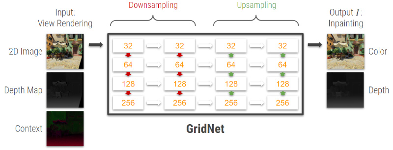
Fig. 41: Inpainting network GridNet
For the color inpainting two loss functions are used to guide the training. The pixel-wise l1 loss Fig. 42 is used to describe the difference between the output $I$ and the ground truth color image $I_{gt}$ . This loss is however not suitable for describing the image content accurately as already mentioned in Fig. 16.
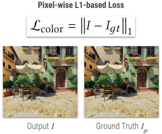
Fig. 42: Color inpainting: pixel-wise l1 loss
For this reason another loss function is used to more accurately describe similar images, the perceptual l2 loss Fig. 43. This loss function compares the differences in high level features, like the style and the content of an image. To compare the high level features of the color output $I$ and its ground truth image $I_{gt}$ , these has to first fed through a modified VGG-19 network. This VGG-19 network contains only the feature extraction part until the relu4_4 activation layer.
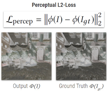
(a) Inputs: activations of the relu4_4 layer from VGG-19
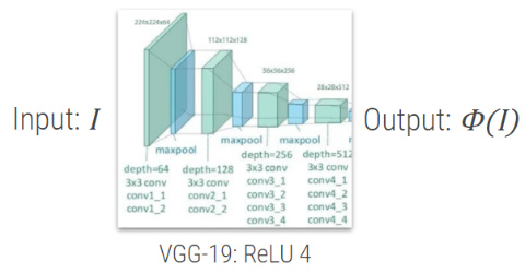
(b) VGG19 relu4_4 layer
The loss function for the depth inpainting is $\mathcal{L_{depth}}=0.0001*\mathcal{L_{ord}}+\mathcal{L_{grad}}$ as described in section Depth Estimation Pipeline.
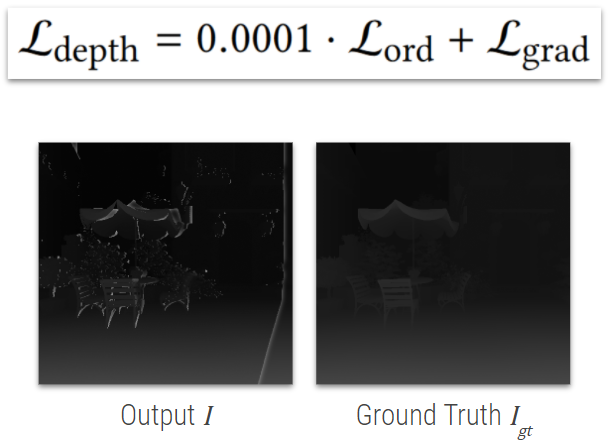
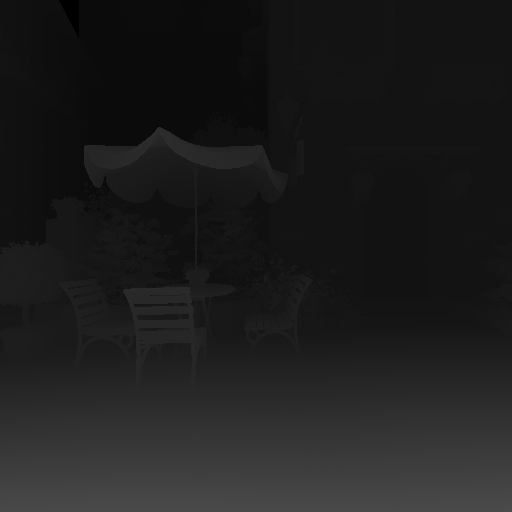
Fig. 44: Depth inpainting: depth loss
The resulting color- and depth inpainting loss function is $\mathcal{L_{inpaint}}=\mathcal{L_{color}}+\mathcal{L_{percep}}+\mathcal{L_{depth}}$ , which will be minimized throughout the training of the inpainting network.
3. Training the Networks
Before triggering the training of the specific networks, the required Python packages needs to be installed. The requirements.txt file contains each Python package which will be needed for the Demo in section 6 and the training of your own models.
!conda install -c conda-forge --file 3d-ken-burns-effect/requirements.txt
!pip install torch torchvision moviepy opencv-contrib-python
!conda install pytorch torchvision cudatoolkit=10.2 -c pytorch --yes
Now it is time to download the synthetic dataset with the help of our download_dataset.py. Note that this step is only necessary when you are running this jupyter notebook locally on your machine. Otherwise the synthetic dataset has already been downloaded to our server. Running this script will automatically download the dataset and create two CSVs which are needed for the training of each network.
The CSVs dataset.csv and dataset_inpainting.csv are used to load random batches during each iteration in the training.
For this purpose a DataLoader class ImageDepthDataset has been implemented. This class takes one of the CSVs and creates a DataLoader which is responsible to load batches from the dataset iteratively throughout the training.
The CSV dataset.csv has the following columns:
| zip_image_path | zip_depth_path | image_path | depth_path | fltFov |
|---|---|---|---|---|
| Path to virtual environment (color information) | Path to virtual environment (depth information) | Path to image | Path to depth map | Field of View for captured sample |
The CSV dataset_inpainting.csv has the following columns:
| zip_image_path | zip_depth_path | image_tl_path | image_tr_path | image_bl_path | image_br_path | depth_tl_path | depth_tr_path | depth_bl_path | depth_br_path | fltFov |
|---|---|---|---|---|---|---|---|---|---|---|
| Path to virtual environment (color information) | Path to virtual environment (depth information) | TL image path | TR image path | BL image path | BR image path | TL depth path | TR depth path | BL depth path | BR depth path | Field of View for captured sample |
Each row of a CSV contains the information of where to load a sample from the synthetic dataset, which is loaded by the class ImageDepthDataset. During the training loop this class will be invoked to retrieve a batch of samples.
Set the path in which you want to download the synthetic dataset:
In order to start the download run the following cell (required if notebook is run on your local machine):
dataset_path = "DESTINATION_PATH" # replace "DESTINATION_PATH" with e.g.: "~/Desktop" or "C:\Users\name\Desktop"
#!python 3d-ken-burns-effect/scripts/download_dataset.py --path {dataset_path} --csv
Implementing a custom Dataset class in Pytorch e.g. ImageDepthDataset requires the following:
- A CSV file containing the information about your dataset. Each row in the CSV contains information for the
DataLoaderwhere your data is located on your machine and how it can be obtained during the training. - An
__init__method taking the path to the CSV file and additional information specific for your use case. Usually Pythonpandasis used to create aDataFramefrom the provided CSV file in order to easily access each row. - A
__len__method which returns the total amount of rows of thepandas’DataFrameobject. - A
__getitem__method which returns a batch of samples. This method can be invoked from the initializedDataLoaderin the training loop. For this purpose your customDatasetclass should include a method likeget_train_valid_loader.
More details can be found in the ImageDepthDataset class.
3.1 Depth Estimation
The Initial Depth Estimation Training notebook contains the scripts for starting the training of the Depth Estimation network.
3.2 Depth Refinement
The Depth Refinement Training notebook contains the scripts for starting the training of the Depth Refinement network.
3.3 Context Extractor and Inpainting Networks
The Context Extractor and Inpainting Networks Training notebook contains the scripts for starting the training of the Context Extractor and Inpainting networks.
4. Results
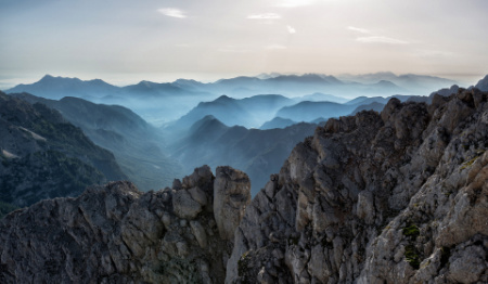

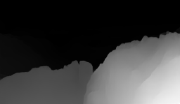


We will compare Niklaus et al and our results which is illustrated in Fig. 45:
(b) Depth Estimation:
Our model is able to detect object boundaries more accurately. The mountain in the foreground is clearly separated from the mountains in the background. However our model assigns higher depth information values for objects in the foreground which results in a brighter depth map as compared to Niklaus et al.
(c) Depth Adjustment:
For the provided input image the depth adjustment process does not seem to apply any visible changes.
(d) Depth Refinement:
The result from Niklaus et al is significantly better than our result. Our result fails to upsample the estimated depth map properly, due to the fact, that we upsampled the training data by a factor of 2 instead of 4. The optimal training process which Niklaus et al. used was the following:
- dimension of ground truth color image or depth map is set to 512 x 512 pixels
- downsampled input color image/depth map obtained from ground truth respectively is set to 128 x 128 pixels
- the U-Net tries to upsample the downsampled training data by a factor of 4
Unfortunately we have trained our refinement model to upsample images by a factor of 2 (256 x 256 pixels to 512 x 512 pixels). This is why our model fails to upsample a high-resolution depth map which is pixelated and thus fails to refine object boundaries properly.
(e) 3D Ken Burns Effect:
Our result is able to detect fine granulated object boundaries in comparison to Niklaus et al. However artifacts at object boundaries are present since the refinement model outputs an pixelated depth map, which fails to separate the foreground from the background precisely.
5. Problems
Depth Estimation
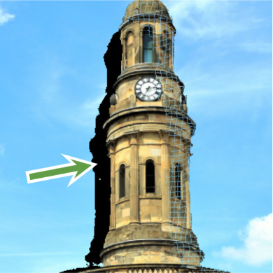
Although Niklaus et al. new method is able to produce depth estimates with little or no distortion, the results may still not be able to predict accurate depth maps for extremely difficult cases such as reflective surfaces or very thin structures, as we can see in the following two images. Since the images are at a relatively low resolution when depth estimation is performed, these errors still happen at times and are hard to eliminate.
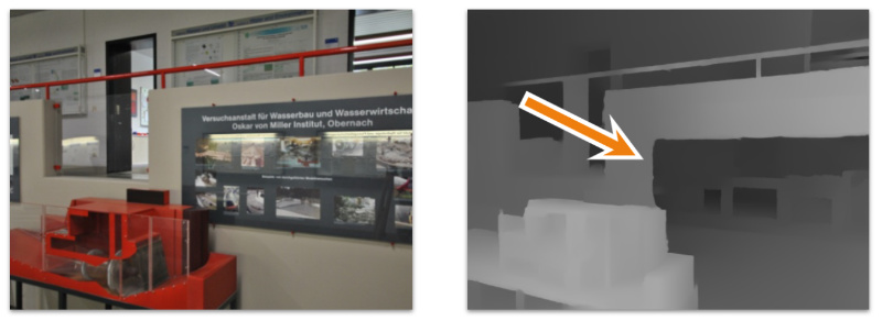
Fig. 46: Example of a thin structure
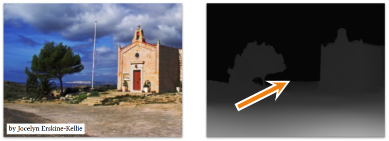
Fig. 47: Example of a reflective surface
Depth Adjustment
Another limitation of their pipeline is the dependency upon other networks such as Mask R-CNN. If they are unable to provide clear results, it is virtually impossible to perform an accurate depth adjustment. One such case can be observed in the image below, where Mask R-CNN provided an inaccurate segmentation mask for the deer on the right and it therefore gets cut off when trying to perform the final 3D Ken Burns Effect.
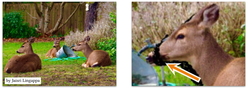
Fig. 48: Example of inaccurate segmentation masks
Color- and depth inpainting
Finally, Niklaus et al. state that while their joint color- and depth inpainting method is an intuitive approach in order to extend the estimated scene geometry, it was so far only monitored on their synthetic training data, which can sometimes create artifacts when the given input differs too much from the training data. In the image below, we can see that the inpainting result lacks texture and is darker than expected.
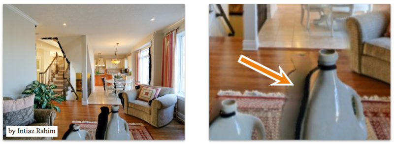
Fig. 49: Example of overfitting on synthetic training data
6. Demo
In the following demo you can choose between five different images and create the 3D Ken Burns Effect yourself.
import os
from matplotlib import pyplot as plt
import cv2
from IPython.display import Video
os.chdir('3d-ken-burns-effect')
The following cell lists the available images from which you can choose one to create the effect.
print('Available images:\n')
for f in os.listdir('../images'):
    print(f'\t{f}')
Available images:

	corridor.jpg
	taxi.jpg
	alpen.jpeg
	rice.jpg
	doublestrike.jpg
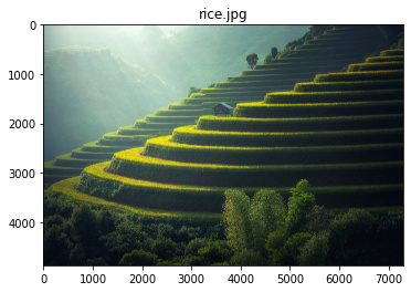
Select one image and change image_path in next cell accordingly.
The selected image will be loaded and displayed.
image_path = "../images/rice.jpg"
video_path = "../videos/video.mp4"
image = cv2.imread(image_path)
image = cv2.cvtColor(image, cv2.COLOR_BGR2RGB)

plt.imshow(image)
plt.title(image_path.split('/')[-1])
plt.show()
The following cell triggers the calculation of the 3D Ken Burns Effect. After completion the generated video will be available for display.
!python autozoom.py --in {image_path} --out {video_path}
Moviepy - Building video ../videos/video.mp4.
Moviepy - Writing video ../videos/video.mp4

Moviepy - Done !
Moviepy - video ready ../videos/video.mp4
Resulting video:
7. References
[1] S. Niklaus, L. Mai, J. Yang, and F. Liu. 2019. 3D Ken Burns Effect from a Single Image. arXiv/1909.05483v1 (2019)
[2] Zhengqi Li, Noah Snavely. 2018. MegaDepth: Learning Single-View Depth Prediction from Internet Photos. arXiv/1804.00607 (2018)
[3] Benjamin Ummenhofer, Huizhong Zhou. 2017. DeMoN: Depth and Motion Network for Learning Monocular Stereo. arXiv/1612.02401 (2017)
[4] Penta, Sashi Kumar. 2005. Depth Image Representation for Image Based Rendering. Diss. International Institute of Information Technology Hyderabad, India, 2005. http://wwwx.cs.unc.edu/~sashi/MSThesis.pdf (2005)
[5] Aashutosh Pyakurel. Planar and Spherical Projections of a Point Cloud (Using Open3D). blog.ekbana.com. https://blog.ekbana.com/planar-and-spherical-projections-of-a-point-cloud-d796db76563e (accessed May. 17, 2020)